Background Material:

It is highly recommended that the reader work through the introductions to single variable calculus and multivariable calculus as a supplement to this section. These materials make accessible the most fundamental aspects of calculus needed to get a firm grasp on gradient-based learning. Even if you are already familiar with calculus, these sections also provide an introduction to automatic differentiation, which will be a critical technology for us moving forward.

Automatic Differentiation

In the previous section, we identified the gradient descent algorithm as a simple but powerful method by which we can optimize a mathematical model’s ability to make reliable predictions about data. We do so by searching for the model parameter values that minimize a loss function, \(\mathscr{L}\), which is responsible for comparing our model’s outputs (i.e. it’s “predictions) against the desired values.

At risk of stating the obvious, performing gradient descent requires that we are able to evaluate \(\vec{\nabla} \mathscr{L}\) - the gradient of our loss function - for any particular input values for the loss function. With the simple examples that we considered in the previous section, we did this by explicitly deriving all of the relevant partial derivatives of \(\mathscr{L}\), \(\begin{bmatrix} \frac{\partial \mathscr{L}}{\partial w_1} & \frac{\partial \mathscr{L}}{\partial w_2} & \cdots & \frac{\partial \mathscr{L}}{\partial w_M} \end{bmatrix}\), by hand. Keep in mind that each of these partial derivatives is itself a function. We then evaluated those partial derivatives, and thus evaluated \(\vec{\nabla} \mathscr{L}\), using our model’s current parameter values by plugging them into these equations. This process worked fine for these simple examples, but we will soon find that deriving each \(\frac{\partial \mathscr{L}}{\partial w_i}\) by hand to be untenable as our mathematical models, and thus \(\mathscr{L}\), begin to grow in complexity.

Fortunately, the recent surge of interest in neural networks and gradient-based learning methods has led to development of popular and highly-powerful automatic differentiation libraries, such as PyTorch, TensorFlow, JAX, and Zygote. These “autodiff” libraries are able to evaluate the derivatives of arbitrary compositions of mathematical functions, such as polynomials, exponentials, and trigonometric functions. These libraries can handle enormously complex functions of many (millions) of variables; the derivatives of such functions would be totally intractable for us to evaluate by-hand.

In this course, we will be making frequent use of the autodiff library called MyGrad, which is designed to behave just like NumPy, but with auto-differentiation added on top. If you already have NumPy installed in your Python environment, you can simply install MyGrad with:

pip install mygrad

The goal of this section is to familiarize ourselves with MyGrad as a tool for performing automatic differentiation, and to give insight into how such a tool works, and how we can wield it effectively. This is a general-purpose capability that will grow in popularity in fields beyond machine learning; you can even use MyGrad to help you with your calculus homework!

An Important Note on Semantics:

To be clear: most automatic differentiation libraries do not produce derivatives of functions. Recall that the derivative of a function is another function; an autodiff library does not produce a symbolic representation of a new function as its output. Instead, an autodiff library can evaluate the derivative(s) of a function at a given input, producing the number(s) that represents the instantaneous slope of the function at that point. Thus, it is more appropriate to say that these autodiff libraries can tell us the instantaneous slope of any function at any point, more so than saying that they can “take the derivative” of any function.

Automatic Differentiation at a Glance

Let’s not dawdle any longer; it is time to see some automatic differentiation in action. Suppose that we have the function

\begin{equation} f(x, y) = xy + x^2 \end{equation}

and that we want to evaluate the first-order partial derivatives of \(f\) at \((x=2, y=4)\). Let’s evaluate these by hands so that we can know what to expect from our autodiff library. The relevant partial derivatives of \(f\) are

\begin{align} \frac{\partial f}{\partial x} &= y + 2x\\ \frac{\partial f}{\partial y} &= x \end{align}

Evaluated at \((x=2, y=4)\) gives:

\begin{align} \frac{\partial f}{\partial x}\big|_{x=2, y=4} &= 4 + 2(2) = 8\\ \frac{\partial f}{\partial y}\big|_{x=2, y=4} &= 2 \end{align}

To compute these derivatives in MyGrad, we need only compute \(f\) at the point(s) of interest; we can then instruct MyGrad to compute the derivatives of \(f\). In order for MyGrad to keep track of the mathematical operations that we are using, we must represent our variables of interest using mygrad.Tensor objects (more on these later).

# Defining x and y, and computing f(x, y)

>>> import mygrad as mg
>>> x = mg.tensor(2.0)
>>> y = mg.tensor(4.0)
>>> f = x * y + x ** 2  # computes f(2, 4)
>>> f # stores f(2, 4) as a mygrad-tensor
Tensor(12.)

The MyGrad-tensor f stores not only the value of \(f(2, 4)\) but also the mathematical operations that were used to compute this value. With this information, we can instruct MyGrad to compute the derivatives of \(f\) with respect to each of its variables - evaluated at the variable’s specific value. We do this by calling the method f.backward() (“backward” is short for “backpropagation” which is the particular automatic differentiation algorithm that MyGrad employs).

# Invoking autodiff, specifically backpropagation
#
# This says: "evaluate all of the derivatives of `f` with
# respect to all of the variables that `f` depends on"
#
>>> f.backward()  # this method doesn't return any value

The derivatives are stored in each of the respective tensors, in the attribute Tensor.grad

# Accessing the derivatives of `f`, stored in the `Tensor.grad`
# attribute. These are always stored as NumPy arrays.
>>> x.grad  # stores df/dx @ x=2, y=4
array(8.)

>>> y.grad  # stores df/dy @ x=2, y=4
array(2.)

Voilà! We have officially used automatic differentiation to evaluate the derivatives of a function. Note that we didn’t need to know any calculus or write down any derivatives to achieve this; all we needed to do was use evaluate the function itself while using MyGrad’s Tensor object to represent our variables. From there, everything else was… automatic.

MyGrad is capable of handling much more complex and interesting functions than this; it will behoove us to familiarize ourselves more thoroughly with this library.

An Introduction to MyGrad

NumPy is the cornerstone for nearly all numerical and scientific computing software in Python, and thus it is desirable for us to spend our time focused on learning NumPy rather than splitting our attention across multiple array-math libraries. For this reason, MyGrad was specifically designed to to act and feel just like NumPy. Thus, if you want to get good at using MyGrad, you should spend most of your time mastering NumPy!.

The crux of MyGrad is the Tensor object. This is analagous to NumPy’s ndarray, as it:

can store N-dimensional array data, which can be manipulated (e.g. reshaped, transposed, etc.)
supports both basic indexing (accessing elements and subsections of tensor), advanced indexing (accessing arbitrary collections of elements from the tensor)
permits convenient vectorized operations, which obey NumPy’s broadcasting semantics
mirrors NumPy’s mechanism for providing views of data and in-place updates on data

What distinguishes the Tensor is that designed to support all of these features, plus it enables automatic differentiation through any mathematical operations that involve tensors.

If you are already at least familiar with each of the above concepts, then you are already well-along your way to being a competent MyGrad user! If these aren’t ringing a bell, then it is strongly recommended that you review the NumPy module from Python Like You Mean It.

Creating and Using Tensors

A Tensor must be provided the array data that it is to store. This can be a single number, a sequence of numbers, a NumPy array, or an existing tensor.

# Creating MyGrad Tensor instances
>>> import mygrad as mg
>>> import numpy as np

# Making a 0-D tensor from a float
>>> mg.tensor(2.3)
Tensor(2.3)

# Making a shape-(3,) tensor of 32-bit floats from a list
>>> mg.tensor([1.0, 2.0, 3.0], dtype=np.float32)
Tensor([1., 2., 3.], dtype=float32)

# Making a shape-(3, 3) tensor from a a numpy array
>>> arr = np.ones((3, 3))
>>> mg.tensor(arr)
Tensor([[1., 1., 1.],
        [1., 1., 1.],
        [1., 1., 1.]])

# creating a shape-(9,) tensor and reshaping
# it into a shape-(3, 3) tensor
>>> x = mg.arange(9.)
>>> x
Tensor([0., 1., 2., 3., 4., 5., 6., 7., 8.])
>>> x.reshape(3, 3)
Tensor([[0., 1., 2.],
        [3., 4., 5.],
        [6., 7., 8.]])

Note that MyGrad uses NumPy’s data-type system exactly so we can pass, e.g., np.float32 anywhere there is a dtype argument in a MyGrad function to tell that function to return a tensor that stores 32-bit floats.

Tensor-Creation Functions

MyGrad provides a whole suite of tensor-creation functions, which exactly mimic their NumPy counterparts. These can be used to conveniently create tensors of specific shapes and with specific values as their elements.

# Demonstrating some of MyGrad's tensor-creation functions

# Create a shape-(10,) tensor of subsequent integer-valued floats 0-9
>>> mg.arange(10.)
Tensor([0., 1., 2., 3., 4., 5., 6., 7., 8., 9.])

# Create a shape-(2, 3, 4) tensor of 0s
>>> mg.zeros((2, 3, 4))
Tensor([[[0., 0., 0., 0.],
         [0., 0., 0., 0.],
         [0., 0., 0., 0.]],

        [[0., 0., 0., 0.],
         [0., 0., 0., 0.],
         [0., 0., 0., 0.]]], dtype=float32)

# Create a shape-(3, 4) tensor of numbers drawn randomly
# from the interval [0, 1)
>>> mg.random.rand(3, 4)
Tensor([[0.84171912, 0.48059864, 0.68269986, 0.72591644],
        [0.2315483 , 0.04201723, 0.51519654, 0.2711251 ],
        [0.76460016, 0.49148986, 0.2825281 , 0.38161674]])

Reading Comprehension: Tensor creation in MyGrad:

Find a MyGrad function that enables you to create a shape-(15,) tensor of 15 evenly-spaced elements over the interval \([0, \pi]\), and use it to create this tensor. Make the tensor store 32-bit floats instead of the standard 64-bit ones.

Standard Mathematical Operations

In terms of math, MyGrad provides all of the same standard arithmetic, trigonometric, and exponential (etc.) functions as does NumPy. These are vectorized functions that obey NumPy’s broadcasting semantics. That is, unary functions naturally operate element-wise over tensors and binary functions naturally map between corresponding pairs of elements between two same-shape tensors.

# Performing NumPy-like mathematical operation in MyGrad
>>> x = mg.tensor([0.0, 0.25, 0.5, 0.75, 1.0])
>>> y = mg.tensor([[0.],
...                [1.],
...                [2.]])

# computing sine on each element of `x`
>>> mg.sin(x)
Tensor([0.        , 0.24740396, 0.47942554, 0.68163876, 0.84147098])

# broadcast-multiply a shape-(5,) tensor with a shape-(3, 1) tensor
# producing a shape-(3, 5) tensor
>>> x * y
Tensor([[0.  , 0.  , 0.  , 0.  , 0.  ],
        [0.  , 0.25, 0.5 , 0.75, 1.  ],
        [0.  , 0.5 , 1.  , 1.5 , 2.  ]])

# summing the rows of `x * y`
>>> mg.sum(x * y, axis=0)
Tensor([0.  , 0.75, 1.5 , 2.25, 3.  ])

The distinguishing feature here is that all of these mathematical operations support automatic differentiation:

# computing the derivatives of `mg.sum(x * y)`
>>> mg.sum(x * y).backward()
>>> x.grad
array([3., 3., 3., 3., 3.])
>>> y.grad
array([[2.5],
       [2.5],
       [2.5]])

Reading Comprehension: Basic Tensor Math

Given the following shape-(4, 4) tensor

>>> x = mg.tensor([[ 0.,  1.,  2.,  3.],
...                [ 4.,  5.,  6.,  7.],
...                [ 8.,  9., 10., 11.],
...                [12., 13., 14., 15.]])

Using basic indexing, take the natural-logarithm of the 1st and 3rd element in the 3rd-row of x, producing a shape-(2,) result.
Add the four quadrants of x (the top-left 2x2 corner, the top-right, etc.), producing a shape-(2, 2) output.
Compute the mean column of x, producing a shape-(4,) output.
Treating each of the rows of x as a vector, update x in-place so that each row is “normalized” - i.e. so that sum(row ** 2) is 1.0 for each row (thus each vector has become a “unit vector”).

Linear Algebra Operations

There are two essential linear algebra functions, matmul and einsum, provided by MyGrad. (In the future, more of NumPy’s linear algebra functions will be implemented by MyGrad). matmul is capable of performing all the common patterns of matrix products, vector products (i.e. “dot” products), and matrix-vector products. einsum, on the other hand, is a rather complicated function, but it is capable of performing a rich and diverse assortment of customizable linear algebra operations - and MyGrad supports autodiff through all of them! It is worthwhile to take some time to study example usages of einsum.

# Demonstrating matmul. Note that `x @ y` is equivalent to `mg.matmul(x, y)`

# Computing the dot-product between two 1D tensors
>>> x = mg.tensor([1.0, 2.0])
>>> y = mg.tensor([-3.0, -4.0])
>>> mg.matmul(x, y)
Tensor(-11.)

# Performing matrix multiplication between two 2D arrays
# shape-(4, 2)
>>> a = mg.tensor([[1, 0],
...                [0, 1],
...                [2, 1],
...                [3, 4]])

# shape-(2, 3)
>>> b = mg.tensor([[4, 1, 5],
...                [2, 2, 6]])

# shape-(4, 2) x shape-(2, 3) -> shape-(4, 3)
>>> a @ b
Tensor([[ 4,  1,  5],
        [ 2,  2,  6],
        [10,  4, 16],
        [20, 11, 39]])

# Broadcast matrix-multiply a stack of 5 shape-(3, 4) matrices
# with a shape-(4, 2) matrix.
# Produces a stack of 5 shape-(3, 2) matrices
>>> x = mg.random.rand(5, 3, 4)
>>> y = mg.random.rand(4, 2)
>>> mg.matmul(x, y)
Tensor([[[1.58748244, 1.51358424],
         [0.51050875, 0.56065769],
         [0.76175208, 0.83783723]],

        [[1.1523679 , 1.1903295 ],
         [1.14289929, 1.18696065],
         [0.92242907, 1.06143745]],

        [[0.5638518 , 0.6160062 ],
         [1.13099094, 1.13372748],
         [0.33663353, 0.33281849]],

        [[0.52271593, 0.47828053],
         [1.1220926 , 1.14347422],
         [0.978343  , 0.96900857]],

        [[0.96079816, 0.82959776],
         [0.5029887 , 0.39473396],
         [0.83622258, 0.84607976]]])

Reading Comprehension: Get a Load of “Einstein” Over Here

Read the documentation for einsum. Then write an expression using mygrad.einsum that operates on two 2D tensors of the same shape, such that it computes the dot product of each corresponding pair of rows between them. I.e. operating on two shape-\((N, D)\) tensors will produce a shape-\((N,)\) tensor storing the resulting dot-product of each of the \(N\) pairs of rows.

Specialized Functions for Deep Learning

Lastly, MyGrad also provides a suite of functions and utilities that are essential for constructing and training neural networks. These include common deep learning operations like performing convolutions and poolings using \(N\)-dimensional sliding windows, and batch normalization. Also supplied are common activation and loss functions, as well as model-weight initialization schemes. We will make heavy use of these in the coming sections.

(For the more advanced reader, you may have noticed that there is not dense operation among the “layer” operations documented under mygrad.nnet. This is because the standard linear algebra function mygrad.matmul already satisfies this functionality!)

# Performing a "conv-net"-style 2D convolution
>>> from mygrad.nnet import conv_nd

# shape-(1, 1, 3, 3)
>>> kernel = mg.tensor([[[[0., 1., 0.],
...                       [1., 1., 1.],
...                       [0., 1., 0.]]]])

# shape-(1, 1, 5, 5)
>>> image = mg.tensor([[[[ 0.,  1.,  2.,  3.,  4.],
...                      [ 5.,  6.,  7.,  8.,  9.],
...                      [10., 11., 12., 13., 14.],
...                      [15., 16., 17., 18., 19.],
...                      [20., 21., 22., 23., 24.]]]])

# shape-(1, 1, 5, 5) result
>>> conv_nd(image, kernel, stride=1, padding=1)
Tensor([[[[ 6.,  9., 13., 17., 16.],
          [21., 30., 35., 40., 35.],
          [41., 55., 60., 65., 55.],
          [61., 80., 85., 90., 75.],
          [56., 79., 83., 87., 66.]]]])

Running Automatic Differentiation

With a bit of know-how about MyGrad under our belts, let’s mosey through a thorough discussion of automatic differentiation.

MyGrad Bakes Autodiff Into Everything It Does

All of the examples of MyGrad’s mathematical operations laid out above behave identically to their NumPy counterparts in terms of the numerical results that they produce. The difference is that MyGrad’s functions were all designed to provide users with the ability to perform automatic differentiation through each of these operations. We saw this in action at the beginning of this section, in “Automatic Differentiation at a Glance”, but that was before we were familiar with MyGrad.

It is important to note that MyGrad’s Tensor objects were written to “overload” the common arithmetic operators, such as + and *, so that you can use these familiar operators but actually invoke the corresponding MyGrad functions. For example, calling:

tensor_c = tensor_a + tensor_b

will actually call

tensor_c = mg.add(tensor_a, tensor_b)

So that we can perform automatic differentiation through this addition operation. We can read about Python’s special methods to better understand how one can design a class to “overload” operators in this way.

MyGrad Adds “Drop-In” AutoDiff to NumPy

MyGrad’s functions are intentionally designed to mirror NumPy’s functions almost exactly. In fact, for all of the NumPy functions that MyGrad mirrors, we can pass a tensor to a NumPy function and it will be “coerced” into returning a tensor instead of a NumPy array – thus we can autodifferentiate through NumPy functions!

# showing off "drop-in" autodiff through NumPy functions
>>> import numpy as np
>>> x = mg.tensor(3.)
>>> y = np.square(x)  # note that we are using a numpy function here!
>>> y  # y is a tensor, not a numpy array
Tensor(9.)
>>> y.backward()  # compute derivatives of y
>>> x.grad  # stores dy/dx @ x=3
array(6.)

How does this work? MyGrad’s tensor is able to tell NumPy’s function to actually call a MyGrad function.

So

np.square(mg.tensor(3.))

actually calls

mg.square(mg.tensor(3.))

under the hood. Not only is this convenient, but it also means that you can take a complex function that is written in terms of numpy functions and pass a tensor through it so that you can differentiate that function!

from some_library import complicated_numpy_function
x = mg.tensor(...)
out_tensor = complicated_numpy_function(x)
out_tensor.backward() # compute d(complicated_numpy_function) / dx !

Making it to the Big Leagues:

During this course, we will have grown so comfortable with automatic differentiation and array mathematics that it will be easy for us to graduate to using “industrial-grade” libraries like PyTorch and TensorFlow, which are much more appropriate for doing high-performance work. These libraries are far more sophisticated than is MyGrad (they have millions of dollars of funding and incredible expertise behind them!) and are able to leveraged specialized computer hardware, like GPUs, to perform blazingly-fast computations. In fact, we will turn to PyTorch for some of our capstone project work.

The All-Important `.backward()` Method

The sole method that we need to use to invoke autodiff in MyGrad is Tensor.backward(). Suppose that we have computed a tensor ℒ from other tensors; calling ℒ.backward() instructs MyGrad to compute the derivatives of ℒ with respect to all of the tensors that it depends on. These derivatives are then stored as NumPy arrays in the .grad attribute in each of the respective tensors that preceded ℒ in its computation.

(Note that we are purposefully using the fancy unicode symbol ℒ (U+2112) to evoke an association with the “loss” function \(\mathscr{L}\), whose gradient we will be interested in computing in machine learning problems. That being said, this is purely an aesthetic choice made for this section; MyGrad does not care about the particular variable names that we use.)

Let’s take an example

x = mg.tensor(2.0)
y = mg.tensor(3.0)
f = x * y  # actually calls: `mygrad.multiply(x, y)`
ℒ = f + x - 2  # actually calls `mygrad.subtract(mygrad.add(f, x), 2)`

See that \(\mathscr{L}\) is a function of \(f\), \(x\), and \(y\), and that \(f\) is a function of \(x\) and \(y\). Thus the “terminal” (final) tensor in this “computational graph” that we have laid out can be thought of as the function \(\mathscr{L}(f(x, y), x, y)\).

As described above, calling ℒ.backward() instructs MyGrad to compute all of the derivatives of ℒ. It does this using an algorithm known as “backpropagation”, which we will discuss later. Suffice it to say that MyGrad simply uses the chain rule (reference) to compute these derivatives.

>>> ℒ.backward()  # triggers computation of derivatives of `ℒ`

>>> f.grad  # stores dℒ/df = ∂ℒ/∂f @ x=2, y=2
array(1.)

>>> y.grad  # stores dℒ/dy = ∂ℒ/∂f ∂f/∂y @ x=2, y=2
array(2.)

>>> x.grad  # stores dℒ/dx = ∂ℒ/∂f ∂f/∂x + ∂ℒ/∂x @ x=2, y=2
array(4.)

To re-emphasize the point made above: MyGrad was only able to access the necessary information to compute all of the derivatives of \(\mathscr{L}\) (via the chain rule) because all of our quantities of interest were stored as MyGrad-tensors, and all of the mathematical operations that we performed on them were functions supplied by MyGrad.

Note that x.grad and y.grad together express the gradient of \(\mathscr{L}\), \(\vec{\nabla}\mathscr{L} = \begin{bmatrix} \frac{d \mathscr{L}}{d x} & \frac{d \mathscr{L}}{dy} \end{bmatrix}\), evaluated at \((x=2, y=3)\). These derivatives are now available for use; e.g. we can use these derivatives to perform gradient descent on \(\mathscr{L}\).

Involving any of these tensors in further operations will automatically “null” its derivative (i.e. set it to None)

# Involving a tensor in a new operation will automatically set
# its `.grad` attribute to `None`
>>> x.grad
array(4.)

>>> x + 2  # nulls the grad stored by `x`
Tensor(4.0)

>>> x.grad is None
True

You can also explicitly call Tensor.null_grad() to set that tensor’s .grad attribute back to None

# Demonstrating `Tensor.null_grad()`
>>> y.grad
array(2.)

>>> y.null_grad()  # returns the tensor itself (for convenience)
Tensor(3.)

>>> y.grad is None
True

It is useful to understand how these gradients get cleared since we will need to make repeated use of a tensor and its associated derivative during gradient descent, and thus we will need to discard of a tensor’s associated derivative between iterations of gradient descent.

Reading Comprehension: Some Basic Autodiff Exercises

Given \(x = 2.5\), compute \(\frac{d\mathscr{L}}{dx}\big|_{x=2.5}\) for the following \(\mathscr{L}(x)\)

\(\mathscr{L}(x) = 2 + 3x - 5x^2\)
\(\mathscr{L}(x) = \cos{(\sqrt{x})}\)
Given \(f(x) = x^2\), \(\mathscr{L}(x) = (2 x f(x))^2 - f(x)\) …define f as a separate tensor before computing ℒ.

Reading Comprehension: A Function By Any Other Name (Would Differentiate The Same)

Given \(x = 2.5\), verify that the following pairs of functions yield the same derivatives in MyGrad.

\(\mathscr{L}(x) = xx\) and \(\mathscr{L}(x) = x^2\)
\(\mathscr{L}(x) = e^{\ln x}\) and \(\mathscr{L}(x) = x\)

Constant Tensors and Mixed Operations with NumPy Arrays

An important feature of MyGrad is that you can do mixed operations between its tensors and other array-like objects or numbers. Not only is this convenient, but it also enables us to designate certain quantities in our computations as constants, i.e. as quantities for which we do not need to compute derivatives. For example, in the following calculation MyGrad only computes one derivative, \(\frac{d\mathscr{L}}{dx}\), of a binary function; this enables us to avoid unnecessary computation if we don’t have any use for \(\frac{d\mathscr{L}}{dy}\).

# Demonstrating mixed operations between tensors
# and non-tensors
>>> import numpy as np
>>> x = mg.tensor([1., 2.])
>>> y = np.array([3., 4.])  # this array acts like "a constant"
>>> ℒ = x * y
>>> ℒ.backward()  # only dℒ/dx is computed
>>> x.grad
array([3., 4.])

All of MyGrad’s functions also accept a “constant” argument, which, when specified as True, will cause the creation of a constant tensor. Just like when it encounters a NumPy array or Python number, MyGrad knows to skip the calculation of a derivative with respect to a constant tensor. We can check the Tensor.constant attribute to see if a tensor is a constant or not.

# Demonstrating the use of a constant Tensor
>>> import numpy as np
>>> x = mg.tensor([1., 2.])
>>> y = mg.tensor([3., 4.], constant=True)

>>> x.constant
False
>>> y.constant
True

>>> ℒ = x * y
>>> ℒ.backward()  # only dℒ/dx is computed
>>> x.grad
array([3., 4.])
>>> y.grad is None
True

Operations only involving constants and constant tensors will naturally create constant tensors.

# Operations involving only constants will produce a constant
>>> out = mg.Tensor([1.0, 2.0], constant=True) + mg.Tensor([3.0, 4.0], constant=True)
>>> out.constant
True

And calling .backward() on a constant tensor will not do anything at all!

# calling `.backward()` on a constant has no effect
>>> out.backward()
>>> out.grad is None

Constants vs. Variables: Why all the fuss?

The semantics of constants versus variable tensors are important because we will often encounter situations wherein we do not need the derivatives for all of the quantities involved in a computation, and that needlessly calculating them would actually be very costly. Consider the case of optimizing the parameters for a machine learning model via gradient descent. As we discussed, that involves computing each \(\frac{d\mathscr{L}}{dw_i}\) for the expression

\begin{equation} \mathscr{L}\big(w_1, ..., w_M ; (x_n, y_n)_{n=0}^{N-1}\big) \end{equation}

Note that we do not need to compute each \(\frac{d\mathscr{L}}{dx_i}\), which represents the derivative of our loss function with respect to each datum in our dataset. If we were optimizing some computer vision model, calculating each \(\frac{d\mathscr{L}}{dx_i}\) would be tantamount to calculating a derivative associated with each pixel of each image in our dataset. Very expensive indeed!

Thus, in MyGrad, we can simply express each \(w_i\) as part of a (variable) tensor, and express each \(x_i\) as part of a NumPy array (or constant tensor), thus when we invoke autodiff on \(\mathscr{L}\big(w_1, ..., w_M ; (x_n, y_n)_{n=0}^{N-1}\big)\) MyGrad will naturally avoid computing any unnecessary derivatives.

Under the Hood of MyGrad’s Tensor (Just a NumPy Array)

It is useful to know that MyGrad isn’t doing anything too fancy under the hood; each Tensor instance is simply holding onto a NumPy array, and is also responsible for keeping track of the mathematical operations that the array was involved in. We can access a tensor’s underlying array via the .data attribute:

# Accessing a tensor's underlying NumPy array...
>>> x = mg.arange(4.)
>>> x
Tensor([0., 1., 2., 3.])

# via `Tensor.data`
>>> x.data
array([0., 1., 2., 3.])

# via `numpy.asarray` and `mygrad.asarray`
>>> np.asarray(x)
array([0., 1., 2., 3.])

>>> mg.asarray(x)
array([0., 1., 2., 3.])

It is useful to keep the intimate relationship between a MyGrad tensor and an underlying NumPy array in mind because it reminds us of how similar these libraries are, and it informs our intuition for how tensors behave. Furthermore, this will prove to be an important technical detail for when we perform gradient descent, where we will want to update directly the data being held by the tensor.

Gradient Descent with MyGrad

Without further ado, let’s leverage automatic differentiation to perform gradient descent on a simple function. To stick with a familiar territory, we will once again perform gradient descent on the simple function \(\mathscr{L}(w) = w^2\). This will match exactly the gradient descent example the we saw in the previous example, only here we will not need to write our the derivative of \(\mathscr{L}(w)\) or evaluate it manually. Instead, by making sure that we store the value representing \(w\) as a MyGrad tensor, and use it to calculate \(L(w)\), we will be able to leverage autodiff.

Recall that we will be updating \(w\) according to the gradient-based step

\begin{equation} w_{\mathrm{new}} = w_{\mathrm{old}} - \delta \frac{\mathrm{d}\mathscr{L}}{\mathrm{d}w}\big|_{w_{\mathrm{old}}} \end{equation}

Picking \(w = 10\) as a starting point, using the learning rate \(\delta=0.3\), and taking five steps, let’s search for the minimum of \(L\). One thing to note here is that we will update the NumPy array underlying the tensor w directly for the gradient-based update.

# Performing gradient descent on ℒ(w) = w ** 2
w = mg.Tensor(10.0)
learning_rate = 0.3
num_steps = 10
print(w)

for step_cnt in range(num_steps):
    ℒ = w ** 2    # compute L(w)
    ℒ.backward()  # compute derivative of L
    w.data -= learning_rate * w.grad  # update w via gradient-step
    print(w)

Tensor(10.)
Tensor(4.)
Tensor(1.6)
Tensor(0.64)
Tensor(0.256)
Tensor(0.1024)
Tensor(0.04096)
Tensor(0.016384)
Tensor(0.0065536)
Tensor(0.00262144)
Tensor(0.00104858)

See that the gradient descent algorithm is steadily guiding use towards the global minimum \(w = 0\), and we didn’t even need to do any calculus on our own!

The line of code that we wrote to represent the gradient-step,

w.data -= learning_rate * w.grad

might be a little more nuanced than one might have expected. We could have instead written

w = w - learning_rate * w.grad

which more closely aligns with the mathematical equation written above. That being said, the former equation has two benefits, both in terms of optimizing computational speed and both deriving from the fact that we are operating directly on the NumPy array stored by w via `w.data:

The form w.data -= learning_rate * w.grad involves only NumPy arrays, thus we do not need to pay the extra computational overhead incurred by MyGrad’s tracking of mathematical operations.
Using the operator -= invokes an augmented update on the data held by w, this means that the computer can directly overwrite the memory associated with w.data instead of allocating a new array and then replacing w.data with it.

Neither of these points really matter for this extremely lightweight example, but they will make more of a difference when we are making many updates to numerous, large arrays of data, which will be the case when we are tuning the parameters of a neural network. Towards that end, be sure to carefully complete the following exercise…

Reading Comprehension: Writing a Generic Gradient-Update Function:

Complete the following Python function, which is responsible for taking an arbitrary collection (e.g. a list) of MyGrad tensors, which are assumed to already store their relevant gradients, and perform a gradient-step on each one of them. That is, assume that, outside of this function, ℒ has already been computed and ℒ.backward() was already invoked so that now all that is left to be done is perform the gradient-based step on each tensor.

This function will be a very useful utility for when you are optimizing a function involving multiple different variables.

(Hint: this should be a very brief function… much shorter than its docstring)

def gradient_step(tensors, learning_rate):
    """
    Performs gradient-step in-place on each of the provides tensors
    according to the standard formulation of gradient descent.

    Parameters
    ----------
    tensors : Union[Tensor, Iterable[Tensors]]
        A single tensor, or an iterable of an arbitrary number of tensors.

        If a `tensor.grad` is `None`for a specific tensor, the update on
        that tensor is skipped.

    learning_rate : float
        The "learning rate" factor for each descent step. A positive number.

    Notes
    -----
    The gradient-steps performed by this function occur in-place on each tensor,
    thus this function does not return anything
    """
    # YOUR CODE HERE

Tensors as Collections of Scalar Variables

Thus far we have focused on equations involving scalars, like Tensor(2.0), which are zero-dimensional tensors. This was done intentionally, since we are most comfortable with thinking of equations that only involve scalars, such as \(f(x) = x^2\); we intuitively know that \(x\) represents a single number here. That being said, the Tensor object was clearly designed to be able to represent an \(N\)-dimensional array of data. How, then, are we to interpret the .grad attribute associated with a multidimensional tensor? The answer, generally, is that each element of a tensor is to be interpreted as a scalar-valued variable.

Consider, for example, the following calculation

>>> tensor = mg.tensor([2.0, 4.0, 8.0])
>>> arr = np.array([-1.0, 2.0, 0])
>>> ℒ = (arr * tensor ** 2).sum()
>>> ℒ.backward()

What value(s) should we expect to be stored in tensor.grad? Take some time to think about this and see if you can convince yourself of an answer.

Let’s work out what we should expect the gradient to be given the aforementioned prescription: that each element of tensor should be treated like a scalar-valued variable. I.e. we’ll say \(\mathrm{tensor} = [x_0, x_1, x_2]\), then the equation for \(\mathscr{L}\) is

\begin{equation} \mathscr{L} = -1\:(x_0)^2 + 2\:(x_1)^2 + 0\:(x_2)^2 \end{equation}

And tensor.grad will store \(\vec{\nabla}\mathscr{L}\) evaluated at the particular value stored by tensor

\begin{align} \vec{\nabla}\mathscr{L} &= \big[\frac{\mathrm{d}\mathscr{L}}{\mathrm{d}x_0},\frac{\mathrm{d}\mathscr{L}}{\mathrm{d}x_1},\frac{\mathrm{d}\mathscr{L}}{\mathrm{d}x_2}\big]\\ &= \big[-2x_0,\:4x_1,\:0x_0\big]\\ \vec{\nabla}\mathscr{L}\big|_{x_0=2, x_1=4, x_2=8} &= \big[-4,\:16,\:0\big] \end{align}

Indeed this is what we find

>>> tensor.grad
array([-4., 16.,  0.])

Thus the .grad array has a clear correspondence with its associated tensor: if tensor is a N-dimensional tensor that is involved in the calculation of a scalar \(\mathscr{L}\) (and assuming that we invoked ℒ.backward()), then t.grad is an array of the same shape as tensor that stores the corresponding derivatives of \(\mathscr{L}\).

That is, given that we think of an element of a tensor to be a scalar-valued variable

\begin{equation} \text{tensor}[i_1, \dots, i_N] \rightarrow x_{i_1, \dots, i_N} \end{equation}

then the corresponding element of the associated gradient is the derivative involving that variable

\begin{equation} \text{tensor.grad}[i_1, \dots, i_N] \rightarrow \frac{\mathrm{d}\mathscr{L}}{\mathrm{d} x_{i_1, \dots, i_N}}\\ \end{equation}

Reading Comprehension: Tensors as Collections of Scalar Variables:

Given the shape-\((3, 3)\) tensor

Tensor([[ 2.,  6.,  7.],
        [ 1.,  4.,  9.],
        [10.,  8.,  5.]])

whose elements correspond to \(x_0, x_1, \dots, x_8\), evaluate the derivatives of

\begin{equation} \mathscr{L} = 0x_0 + 1x_1 + \dots + 8x_8 = \sum_{n=0}^8{n x_n} \end{equation}

Reading Comprehension: Descent Down a Parabolic Surface using MyGrad:

(This problem mirrors a reading comprehension question from the previous section on gradient descent, but here we leverage automatic differentiation)

Using automatic differentiation with MyGrad, complete the following Python function that implements gradient descent on the skewed paraboloid \(\mathscr{L}(w_1, w_2) = 2 w_1^2 + 3 w_2^2\).

Note that you should not need to derive/compute the partial derivatives of \(\mathscr{L}\) yourself.

Your calculation of \(\mathscr{L}(w_1, w_2) = 2 w_1^2 + 3 w_2^2\) should be fully vectorized; i.e. you should use a shape-(2,) tensor w to store \([w_1, w_2]\), and perform element-wise operations on it in order to compute \(\mathscr{L}\). Think about what array you can use do element-wise multiplication, but where you are performing (2*, 3*).

Use your gradient_step function to make updates to w.

def descent_down_2d_parabola(w_start, learning_rate, num_steps):
    """
    Performs gradient descent on ℒ(w1, w2) = 2 * w1 ** 2 + 3 * w2 **2 ,
    returning the sequence of w-values: [w_start, ..., w_stop]

    Parameters
    ----------
    w_start : mygrad.Tensor, shape-(2,)
        The initial value of (w1, w2).

    learning_rate : float
        The "learning rate" factor for each descent step. A positive number.

    num_steps : int
        The number subsequent of descent steps taken. A non-negative number.

    Returns
    -------
    Tensor, shape-(2,)
        The final updated values of (w_1, w_2)
    """
    # YOUR CODE HERE

Test your function using the inputs w_start=mg.Tensor([2.0, 4.0]), learning_rate=0.1, and num_steps=10.

Vectorized Autodiff

There was an important caveat made above, which is that we always assume that the “terminus” from which we call .backward() is a scalar. If we call .backward() from a tensor that is not a scalar, then MyGrad acts as if the terminus tensor has first been summed to down a scalar, and then backpropagation is invoked. It is essential that \(\mathscr{L}\) is a scalar so that each \(\frac{\mathrm{d}\mathscr{L}}{\mathrm{d} x_{i_1, \dots, i_N}}\) is also a scalar, and so that tensor and tensor.grad always possess the same shape.

That being said, this mechanism affords us some rather convenient behavior. Consider the following computation:

# a tensor of 100 evenly-spaced elements along [-5, 5]
>>> tensor = mg.linspace(-5, 5, 100)
>>> ℒ = tensor ** 2  # shape-(100) tensor
>>> ℒ.backward()
>>> tensor.grad
array([-10.        ,  -9.7979798 ,  -9.5959596 ,  -9.39393939,
        -9.19191919,  -8.98989899,  -8.78787879,  -8.58585859,
        -8.38383838,  -8.18181818,  -7.97979798,  -7.77777778,
        ...
         8.58585859,   8.78787879,   8.98989899,   9.19191919,
         9.39393939,   9.5959596 ,   9.7979798 ,  10.        ])

Recall that tensor ** 2 simply represents the element-wise application of the square operator, thus \(\mathscr{L}\) is

\begin{equation} \mathscr{L} = \big[x_0 ^2,;\ \dots, \; x^2_{99} \big] \end{equation}

In MyGrad, invoking ℒ.backward() behaves as if we have first summed \(\mathscr{L}\) before invoking .backward(), but note that the terms in this sum are all independent:

\begin{equation} \Sigma{\mathscr{L}} = x_0 ^2 + \dots + x^2_{99} \end{equation}

thus the gradient is simply

\begin{equation} \vec{\nabla}(\Sigma{\mathscr{L}}) = \big[2x_0,;\ \dots, \; 2x_{99} \big] \end{equation}

See that the original operation was simply the element-wise square operation, and that the gradient corresponds simply to the element-wise derivative as well. In essence, we performed a vectorized computation of \(f(x) = x ^ 2\) and its derivative \(\frac{\mathrm{d}f}{\mathrm{d}x} = 2x\) at 100 independent values.

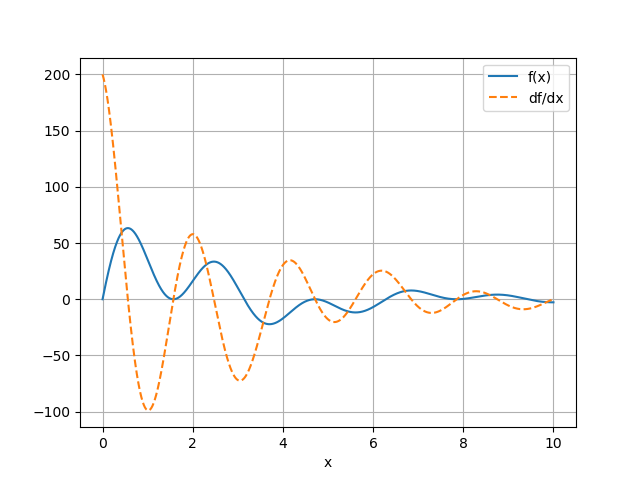
Reading Comprehension: Derivative Plotter:

Complete the following function that leverages vectorized autodiff to plot a function and its derivative over a user-specified domain of values. Refer to this resource for a primer on using Matplotlib.

Note that matplotlib’s functions might not know how to process tensors, so we should pass them arrays instead (recall that tensor.data will return the array associated with a tensor).

Provide labels for the respective plots of func(x) and its derivative, and include a legend.

def plot_func_and_deriv(x, func):
    """ Plots func(x) and dfunc/dx on the same set of axes at the user-specified point
    stored in ``x``.

    Parameters
    ----------
    x : mygrad.Tensor, shape-(N,)
        The positions at which `func` and its derivative will be
        evaluated and plotted.

    func: Callable[[Tensor], Tensor]
        A unary function that is assumed to support backpropagation via MyGrad.
        I.e. calling `func(x).backward()` will compute the derivative(s) of `func`
        with respect to `x`.

    Returns
    -------
    Tuple[Figure, Axis]
        The figure and axis objects associated with the plot that was produced.`l
    """
    # YOUR CODE HERE

Use this utility to plot the function

\begin{equation} f(x) = \sin{(2x)}\; \cos{(x)}\; e^{-x/3} \end{equation}

and its derivative evaluated at 10,000 evenly-spaced points over \([0, 10]\)

Differentiate *The Universe* (Hot-Take Alert):

Presently, automatic differentiation is proving to far more useful than simply being a means for facilitating gradient descent. Indeed the ability to richly measure “cause and effect” through sophisticated computer programs via autodiff is spurring advancements in, and new connections between, fields such as scientific computing, physics, probabilistic programming, machine learning, and others.

Programming languages like Julia are advancing a paradigm known as differentiable programming, in which automatic differentiation can be performed directly on arbitrary code. This is in contrast to using an autodiff library like MyGrad, in which you have to constrain your computer program to specifically use only that library’s functionality, rather than write generic Python code, in order to enjoy the benefits of automatic differentiability. The impact of differentiable programming is that computer programs that were written for specialized purposes - and without heed to any notion of differentiability - can be incorporated into a framework that is nonetheless fully differentiable. Because of this, programs like physics engines, ray tracers, and neural networks can all be combined into a fully differentiable system, and this differentiability can then enable rich new optimizations, simulations, and analyses through these programs.

The new synergies, advancements, and problems resulting from technologies like differentiable programming are being categorized as items in the field of “scentific machine learning”. It is my (the author’s) opinion that the recent advancements in deep learning, which is attributed to neural networks and early automatic differentiation tools, will eventually be seen as a mere prelude to a more staggering impact made across the STEM fields by differentiable programming and scientific machine learning.

Summary and Looking Ahead

The past decade featured the emergence of powerful numerical software libraries that are equipped with the ability to automatically compute derivatives associated with calculations. These are known as automatic differentiation libraries, or “autodiff” libraries. PyTorch and Tensorflow are examples of extremely popular libraries that feature autodiff capabilities.

The “killer” application of autodiff libraries has been to enable the use of gradient descent to optimize arbitrarily-complex mathematical models, where a model is implemented using the tools supplied by an autodiff library so that the derivatives associated with its parameters can be calculated “automatically”. As we will see, this process is very often the driving force behind the “learning” in “deep learning”; that is, to optimize the parameters of a neural network.

We were introduced to MyGrad, which is a simple and ergonomic autodiff library whose primary purpose is to act like “NumPy + autodiff”; in this way we can continue to focusing on developing our NumPy skills with little distraction. Towards this end MyGrad provides a Tensor class, which behaves nearly identically to NumPy’s ndarray class. It’s main difference is that standard mathematical operations using arithmetic operators (+, *, etc.), or using MyGrad’s suite of functions, and involving MyGrad-tensors will be tracked by MyGrad so that derivatives through arbitrary compositions of functions can be computed. Specifically, MyGrad uses an algorithm known as “backpropagation” to perform this automatic differentiation.

Looking Ahead

The next exercise notebook is a very important one; in it we will return to our modeling problem where we selected a linear model to describe the relationship between an NBA player’s height and his wingspan. Before, we found that we could exactly solve for the model parameters (i.e. the slope and y-intercept) that minimize the squared-residuals between our recorded data and our model’s predictions. Now, we will act as if no such analytic solution exists, since this will almost always be the case in “real world” problems. Instead, we will use gradient descent to tune the parameters of our linear model, and we will do this by leveraging MyGrad’s autodiff capabilities to compute the relevant gradients for this optimization process. The procedure that we exercise here will turn out to be almost exactly identical to the process for “training a neural network” using “supervised learning”.

Reading Comprehension Exercise Solutions

Tensor creation in MyGrad: Solution

Find a MyGrad function that enables you to create a tensor of 15 evenly-spaced elements over the interval \([0, \pi]\), and use it to create this tensor. Make the tensor store 32-bit floats instead of the standard 64-bit ones.

mygrad.linspace is the function that generates a tensor of elements evenly spaced over a specified interval.

>>> import mygrad as mg

# Create a shape-(15,) tensor of elements over [0, pi]
>>> mg.linspace(0, mg.pi, 15)
Tensor([0.        , 0.22439948, 0.44879895, 0.67319843, 0.8975979 ,
        1.12199738, 1.34639685, 1.57079633, 1.7951958 , 2.01959528,
        2.24399475, 2.46839423, 2.6927937 , 2.91719318, 3.14159265])

Basic Tensor Math: Solution:

>>> x = mg.Tensor([[ 0.,  1.,  2.,  3.],
...                [ 4.,  5.,  6.,  7.],
...                [ 8.,  9., 10., 11.],
...                [12., 13., 14., 15.]])


# 1. Take the natural-logarithm of the 1st and 3rd element
#    in the 3rd-row of x, producing a shape-(2,) result.
#
# Select the desired row and then use the slice `::2`
# to slice "every other" column - i.e. columns 1 and 3.
>>> mg.log(x[2, 0::2])
Tensor([2.07944154, 2.30258509])

# 2. Add the four quadrants of `x`, producing a shape-(2, 2) output.
#    top-left  top-right    bottom-left  bottom-right
>>> x[:2, :2] + x[:2, -2:] + x[-2:, :2] + x[-2:, -2:]
Tensor([[20., 24.],
        [36., 40.]])

# 3. Compute the mean column of `x`, producing a shape-(4,) output
>>> x.mean(axis=1)
Tensor([ 1.5,  5.5,  9.5, 13.5])

# 4. Treating each of the rows of `x` as a vector, update `x` in-place so
#    that each row is "normalized"
#
# We use /= to perform an in-place division on `x`.
# The `mg.sum(..., keepdims=True)` option makes it convenient to make the
# row-wise magnitudes that we compute broadcast-compatible with x
>>> x /= mg.sqrt(mg.sum(x ** 2, axis=1, keepdims=True))

# Checking the normalization
>>> (x ** 2).sum(axis=1)
Tensor([1., 1., 1., 1.])

Get a Load of “Einstein” Over Here: Solution