Multivariable Calculus: Partial Derivatives & Gradients
This section introduces some concepts from multivariable calculus that will supplement your understanding of gradient descent, which we will also introduce. Namely, this section will provide an explanation of partial derivatives and gradients, extending the idea of the derivative to multivariable functions. We will not need an intimate understanding of gradients moving forward with this course. That being said, it is useful to at least have a cursory understanding of it. Ultimately, however, as you develop a more sophisticated understanding of machine learning, you will want to have a firm grasp on gradients. Since the gradient also pops up all over the place in physics and math, there are many online resources that you can turn to for dedicated lessons on this topic.
What is a Partial Derivative?
If you are comfortable with taking the derivative of a function of a single variable, then partial derivatives are pretty straightforward. Suppose we have a function that depends on two variables:
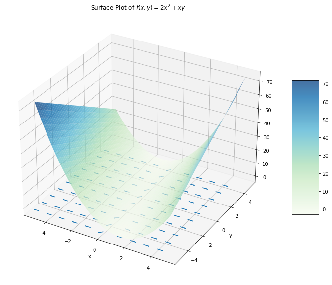
The graph of \(f(x,y)\) would look like a sloping valley, as depicted below.
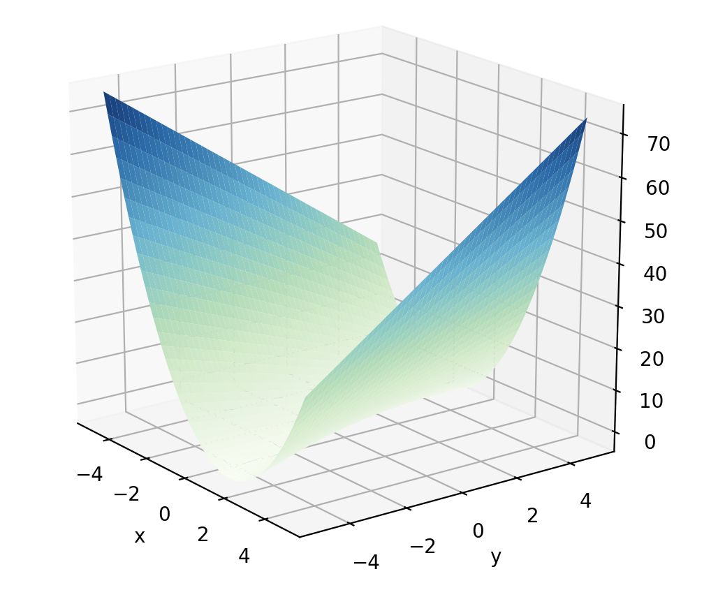
We can walk anywhere along the horizontal plane (in the \(x\) and \(y\) directions), and the value of \(f(x,y)\) tells us our altitude at that point on the valley’s surface.
Now, if this were a single-variable function, the derivative would tell us the instantaneous slope of that function at any and all points. But that is when we can only move along one axis (when \(f\) depends on one variable only). If you were asked stood in a valley and asked “what is the slope of where you are standing?”, it would be natural to respond “in which direction do you mean”? Perhaps the valley is flat along the direction you are facing, whereas the valley slopes upward towards your right (and thus downward to your left). Once we are dealing with functions depending on more than one variable, we must specify the direction along which we are taking our derivative. This is where partial derivatives come into play.
The partial derivative of \(f(x,y)\) with respect to \(x\), denoted \(\frac{\partial f}{\partial x}\), gives us the slope of \(f(x,y)\) along the \(x\)-direction. To accomplish this, we simply take the derivative of \(f(x,y)\) as if \(x\) was the only variable that \(f(x,y)\) depended on (i.e. as if \(y\) were a constant, like the number \(3\)). For our earlier \(f(x,y)\), we can compute the partial derivative with respect to \(x\) as
Notice that, just as the derivative of \(3x\) is \(3\), the partial derivative of the \(xy\) term with respect to \(x\) is \(y\). Furthermore, observe that \(\frac{\partial f}{\partial x}\) is itself a function of both \(x\) and \(y\). This means that the slope of \(f\) along the \(x\)-direction depends on both \(x\) and \(y\). This should make intuitive sense - if I ask you what the slope of the valley is along the \(x\)-direction, your answer should typically depend on where in the valley you are standing.
There is nothing special about \(x\), and so we can also ask for the slope of \(f(x,y)\) along the \(y\)-axis (i.e. take the derivative as if \(y\) was the only variable):
The \(2x^2\) term did not involve \(y\) at all, so its partial derivative with respect to \(y\) is \(0\) (just as the derivative of \(2\) with respect to \(y\) is \(0\)). It turns out that, in this example, \(\frac{\partial f}{\partial y}\) is only a function of \(x\) - I can tell you the slope of \(f(x,y)\) in the \(y\) direction by only knowing where I stand along the \(x\) axis. It should be emphasized that this is merely a feature of this specific function we are working with and will not be generally true.
Reading Comprehension: Finding Partial Derivatives
Find the derivative with respect to each of \(x\), \(y\), and \(z\) of the following function:
These are denoted as \(\frac{\partial f}{\partial x}\), \(\frac{\partial f}{\partial y}\), and \(\frac{\partial f}{\partial z}\), respectively. Which variables, if any, does each partial derivative depend on?
Taking a Derivative Along Any Direction Using the Gradient
Finally, and we can’t give this the full treatment it deserves, what if we want to take the derivative of \(f(x,y)\) along some other direction? Say, we are facing \(45^\circ\) between the \(+x\) and \(+y\) directions, and we want to know the slope of \(f(x,y)\) along this direction. This is where the gradient comes into play. In short, the gradient of \(f(x,y)\) is the vector containing all of the partial derivatives of \(f(x,y)\). In other words, the gradient of \(f(x,y)\) is a vector whose components are the functions
For example, the gradient of our function \(f(x,y)=2x^2+xy\) would be
In the same way that we must plug in values for \(x\) and \(y\) in order to evaluate \(f(x,y)\), we must do the same to evaluate the vector \(\vec{\nabla} f(x,y)\). Evaluating the gradient at the point, say, \((x=1,y=2)\), we find \(\vec{\nabla} f(1,2) = \begin{bmatrix} 6 & 1 \end{bmatrix}\).
Please note that \(f\) could have been a function of \(N\) variables rather than \(2\); the definition of the gradient extends trivially as
Properties of the Gradient
The gradient has a few very important properties that will drive our later applications of it. It will be helpful to be familiar with the dot product before proceeding. Finally, for notational brevity, we will write \(f\) to refer to a multivariable function \(f(x_1,\dots,x_N)\) of \(N\) variables as all the following concepts can be applied in \(N\) dimensions.
Start by noticing that the dot product of \(\vec{\nabla} f(x,y)\) and \(\hat{x}\) yields \(\frac{\partial f}{\partial x}\). Thus taking the dot product of the gradient of \(f(x,y)\) with the \(x\)-unit vector returns the derivative of \(f(x,y)\) along the \(x\)-direction. This generalizes to the important property:
The dot product of \(\hat{u}\) with \(\vec{\nabla} f\) returns the derivative of \(f\) along the direction of \(\hat{u}\). We denote this “directional derivative” as \(\vec{\nabla}_{\hat{u}}f\triangleq\hat{u}\cdot\vec{\nabla}f\).
We can use this fact to prove the second important property about the gradient:
The gradient \(\vec{\nabla} f\) points in the direction of steepest ascent of \(f\) for any and all points.
To see this, consider an \(N\)-D unit vector \(\hat{u}\) that points in the direction of steepest ascent of \(f\) evaluated at a point \(\boldsymbol{p}\). We can find the instantaneous slope at \(\boldsymbol{p}\) in the direction of \(\hat{u}\) by taking the dot product with the gradient \(\vec{\nabla}f\) evaluated at the point \(\boldsymbol{p}\), \(\vec{\nabla}f(\boldsymbol{p})\).
However, we know the dot product is related to the angle between \(\hat{u}\) and \(\vec{\nabla}f(\boldsymbol{p})\) by
Now, we assumed that \(\hat{u}\) points in the direction of steepest ascent, which means that the instantaneous slope at \(\hat{p}\) in the direction of \(\hat{u}\) must be maximal. Since \(\vec{\nabla}_{\hat{u}}f(\boldsymbol{p})\) is this instantaneous slope, we then know that \(\lVert\vec{\nabla}f(\boldsymbol{p})\rVert\cos\theta\) must be maximal. But \(\cos\theta\) is maximized for \(\theta=0\), i.e. when \(\hat{u}\) and \(\vec{\nabla}f(\boldsymbol{p})\) are aligned, meaning that \(\vec{\nabla}f(\boldsymbol{p})\) itself points in the direction of steepest ascent relative to the point \(\boldsymbol{p}\)!
Because of these two properties, the gradient is an extremely useful tool. We can take the derivative of \(f(x,y)\) along an arbitrary direction by writing down the unit vector that points in the desired direction and taking the dot product with the gradient.
Say we wanted to find the derivative of \(f(x,y)=2x^2+xy\) along a line pointing \(45^\circ\) between the positive \(x\) and positive \(y\) directions. One way to visualize this is using a plane along this direction, slicing through \(f(x,y)\):
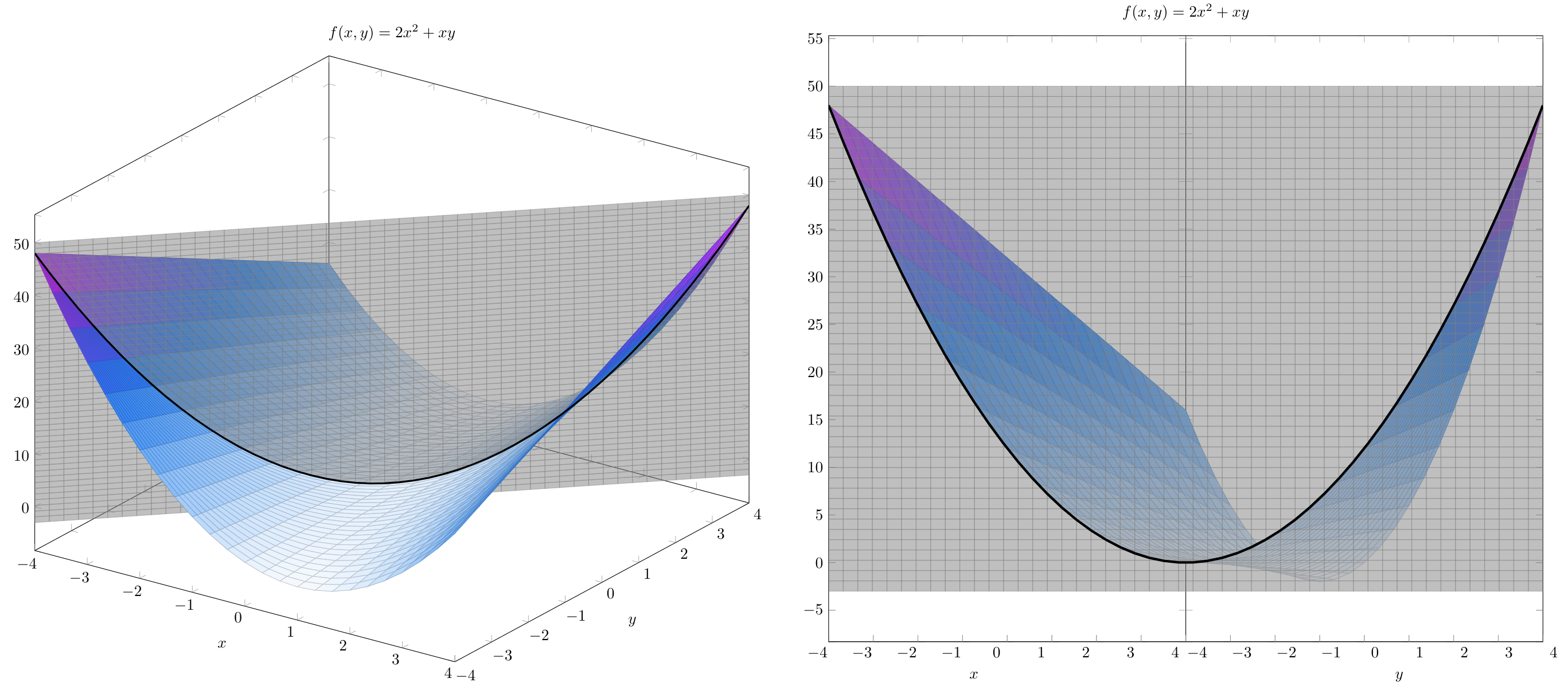
We can write the unit vector that points in the desired direction as
Check that this vector does indeed have a magnitude of 1. And so the derivative of \(f(x,y)\) along the \(\hat{u}\) direction is given by
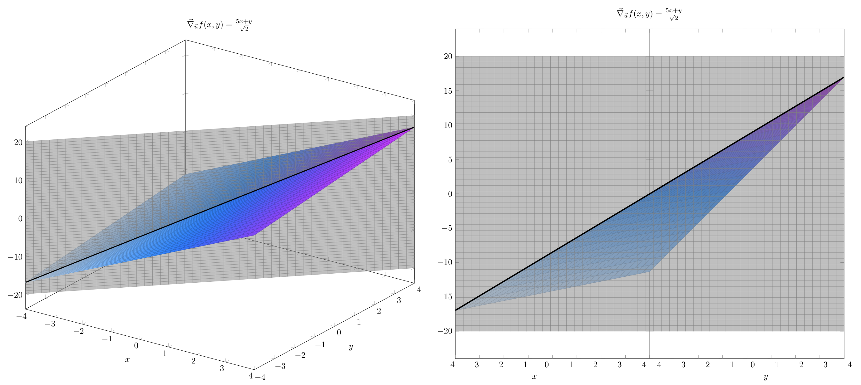
Thus, the function \(\frac{5x+y}{\sqrt{2}}\) tells us the slope of \(f(x,y)\) when we are standing at the point \((x,y)\), facing in the \(\hat{u}\) direction. This derivative can be visualized as
To visualize the gradient, we can think of placing an arrow at every point in the valley directed in the direction of steepest ascent.
For \(f(x,y)=2x^2+xy\), this can be visualized as on the left. The length of each arrow is proportional to the magnitude of the instantaneous slope in the direction of greatest ascent at that point.
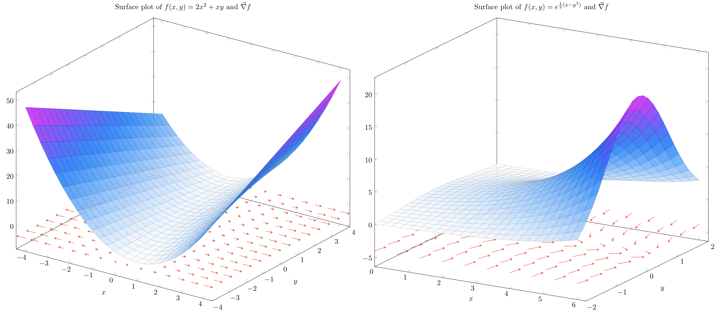
The function on the right was chosen to better illustrate the change in the direction of the gradient at varying values of \(x\) and \(y\). From here it becomes clear: just as if you were standing in a valley, the direction of steepest ascent depends first and foremost on where you are standing.
Reading Comprehension: Applying the Gradient
Find the derivative of \(f(x,y) = 4xy + y^3\) along a line pointing \(30^\circ\) along the \(-x\) and \(+y\) directions (\(150^\circ\) along the \(+x\) and \(+y\) directions). First find \(\vec{\nabla} f(x,y)\) and \(\hat{u}\) and then use these vectors to find the slope of \(f\) in the \(\hat{u}\) direction.
Visualizing the Gradient
The following code generates a surface plot of the function \(f(x,y) = 2x^2 + xy\) and a quiver plot of \(\vec{\nabla}f(x,y)=\begin{bmatrix}4x+y & x\end{bmatrix}\). Run the code in a Jupyter Notebook to see the plot. Change the line Z = 2 * X ** 2 + X * Y to plot some of the other functions we have discussed; note that you should use MyGrad functions (e.g. mg.exp and mg.cos) if needed.
Imagine that you are standing at some point on the surface; notice that the derivative of \(f\), or the slope of the graph where you’re standing, is different depending on the direction you are facing. For example, at the point \((0,0)\), if you are facing the \(+x\) direction the slope is nearly flat, whereas facing the \(+y\) direction there is a very large slope. The gradient of \(f\), or \(\vec{\nabla} f\), points in the direction of steepest ascent for the point it is evaluated at.
[1]:
import numpy as np
import mygrad as mg
from matplotlib import pyplot as plt
from mpl_toolkits.mplot3d import axes3d

%matplotlib inline

fig = plt.figure(figsize=(14, 10))
ax1 = fig.add_subplot(111, projection="3d")

_range = (-5, 5, 0.05)
X, Y = mg.arange(*_range), mg.arange(*_range).reshape(-1, 1)

###
Z = 2 * X ** 2 + X * Y
###

# compute the ∂Z/∂X and ∂Z/∂Y at the
# sampled points in X and Y
mg.sum(Z).backward()

_cmap = plt.get_cmap("GnBu")
plt.xlabel("x")
plt.ylabel("y")
ax1.set_title("Surface Plot of $f(x,y)=2x^2+xy$")

# get underlying numpy arrays for plotting
U = X.grad[::20]
V = Y.grad[::20]
X = X.data
Y = Y.data
Z = Z.data
zeros = np.full_like(Z[::20, ::20], Z.min() - 1e-2)

# reduce the sampling for the quiver plot so that arrows are distinuishable
ax1.quiver(X[::20], Y[::20], zeros, U, V, zeros, length=0.4, normalize=True)

surf = ax1.plot_surface(X, Y, Z, cmap=_cmap, alpha=0.75)
fig.colorbar(surf, ax=ax1, shrink=0.5, aspect=5)
[1]:
<matplotlib.colorbar.Colorbar at 0x212d4162d60>
Minimizing a Function Using Gradient Descent
If \(\vec{\nabla} f\) points in the direction of steepest ascent for a given point, then \(- \vec{\nabla} f\) points in the direction of steepest descent. As we will see, this is exactly the information we need to find a minimum of a function when analytic methods fail.
The analytical method for finding the extrema of a function \(f\) involves setting each partial derivative of the function equal to zero, much like the extrema of a single-variable function are found where the derivative is \(0\). We run into problems, however, when there is no solution to \(\frac{\partial f}{\partial x}=0\), for some variable \(x\). Take the single-variable function \(f(x)=\frac{1}{2}x^2 + e^{-x}\), which can be visualized as
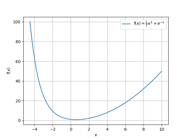
The derivative of \(f(x)\) with respect to \(x\) is \(x-e^{-x}\). Unfortunately, there is no solution in terms of standard functions when we set \(\frac{\mathrm{d}f}{\mathrm{d}x}\) equal to \(0\), but the plot of \(f(x)\) shows that there is indeed a minimum around \(x=0.56\). In this case, it is necessary to use a numerical method to find the extrema.
This is where the gradient comes into play. Starting at any point along our function, we can compute \(\vec{\nabla} f\) to find the instantaneous slope along the direction of steepest ascent at this point. If we want to minimize our function, we ought to move in the opposite direction of the gradient: the direction of greatest descent. We can begin to step towards the location of our minimum by subtracting the gradient of \(f(x)\) at location \(x\) from the value \(x\) itself, making linear approximations of our function in order to move to a location closer to the minimum. It is important to note that a linear approximation is good for a small region around \(x\), but diverges greatly from the function outside of that region. Since the gradient itself can be quite large, we will often need to scale it down, such that we walk in the same direction, but take a much smaller step.
Let’s consider a starting location of \(x=-1\) for our function \(f(x)\). The gradient of our single-variable function is simply the derivative, or \(\vec{\nabla} f(x)=x-e^{-x}\). Evaluating the gradient at \(x=-1\), we have that \(\vec{\nabla} f(-1)=-3.72\). We can subtract this from our current \(x\)-value to arrive at our new location of
We will continue this process iteratively, and now find the gradient at our new location as \(\vec{\nabla} f(2.72)=2.65\). Taking our next step, we arrive at
Although we originally overshot it, subsequent iterations of this will lead us closer and closer to the minimum around \(x=0.56\).
We can also see this process work for our previous multivariable example \(f(x,y) = 2x^2 + xy\), which has a “valley” of minima at \(x=0\) for all values of \(y\). Recall that \(\vec{\nabla} f(x,y) = \begin{bmatrix} 4x+y & x \end{bmatrix}\). Starting (somewhat arbitrarily) at the point \((x=1,y=2)\), we have that \(\vec{\nabla} f(1,2) = \begin{bmatrix} 6 & 1 \end{bmatrix}\). We can subtract each partial derivative in the gradient from its corresponding current \(x\)- or \(y\)-value,
Unfortunately, we’ve gone strayed pretty far from the minima at \(x=0\), because our gradient was relatively large. To accommodate this, we can scale our gradient down by multiplying it with a small, positive scalar; since scalar multiplication has the affect of changing the length of a vector, while maintaining its direction, this will allow us to modify the size of the steps we take.
Let’s take another step, by first evaluating the gradient at \((x,y)_\text{new}\) as \(\vec{\nabla} f(-5,1) = \begin{bmatrix} -19 & -5 \end{bmatrix}\). Before subtracting off the gradient, however, we will multiply our gradient by \(0.1\):
Clearly we have made better progress when we first scaled our gradient; we see that \(x_\text{new}\) is now slightly closer to \(x=0\), as opposed to much farther from it. Check that had we not scaled our gradient down, this step would have taken us to the point \((x=14,y=6)\), quite far from the minima. Without scaling down the gradient, we tend to take big steps back and forth and fail to effectively narrow in on a specific minimum. This makes sense mathematically as well: remember that we are simply making linear approximations, which are only valid in small intervals surrounding the point we evaluate at.
This iterative process of finding the minimum of a function numerically is known as gradient descent, which has the following general form for functions of \(n\) variables
where \(\vec{\nabla} f (x_{1_\text{old}}, x_{2_\text{old}}, \cdots, x_{N_\text{old}})\) is the gradient of \(f\) evaluated at \(\begin{bmatrix} x_1 & x_2 & \cdots & x_N \end{bmatrix}_\text{old}\) and \(\delta\) is a small, positive, real number called the step size.
Reading Comprehension: Stepping Through Gradient Descent
Re-do the first two steps of gradient descent by hand for \(f(x,y) = 2x^2 + xy\) with a step size of \(\delta=0.1\).
Reading Comprehension: Programming Single-Variable Gradient Descent
Write a program that performs gradient descent on the function \(f(x)=\frac{1}{2}x^2 + e^{-x}\). Your program should take a starting coordinate \(x\) and a number of iterations \(n\). Try running your algorithm for a few hundred iterations to see if you end up near the minimum around \(x=0.56\). Experiment with \(\delta\) to see if there is a value that is small enough to avoid overshooting the minimum but large enough to efficiently narrow in on it (avoiding an excessive number of iterations).
Autodifferentiation with Multivariable Functions
Autodifferentiation libraries, like MyGrad, can be used to compute the partial derivatives of multivariable functions.
# using mygrad to compute the derivatives of a multivariable function

import mygrad as mg

>>> x = mg.tensor(3)
>>> y = mg.tensor(4)

>>> f = 2 * (x ** 2) + x * y
>>> f.backward()

# stores ∂f/∂x @ x=3, y=4
>>> x.grad
array(16.)

# stores ∂f/∂y @ x=3, y=4
>>> y.grad
array(3.)
For the chosen \(f(x,y)\), we know that \(\vec{\nabla}f=\begin{bmatrix}4x+y & x\end{bmatrix}\). Evaluating \(\vec{\nabla}f\) at \((x=3,y=4)\),
We can now see that x.grad stores \(\frac{\partial f}{\partial x}\big|_{x=3,y=4}\) and y.grad stores \(\frac{\partial f}{\partial y}\big|_{x=3,y=4}\).
Reading Comprehension: Programming Multivariable Gradient Descent
Write a program that performs gradient descent on the function \(f(x, y)=2x^2 + 4y^2 + e^{-3x} + 3e^{-2y}\). Your program should take starting coordinates \(x\) and \(y\) and a number of iterations \(n\). Try running your algorithm for a few hundred iterations to see if you end up near the minimum around \(x=0.3026, y=0.3629\). Experiment with \(\delta\) to see if there is a value that is small enough to avoid overshooting the minimum but large enough to efficiently narrow in on it (avoiding an excessive number of iterations).
Warning: Make sure that when you are updating the value of Tensors, you perform the update to Tensor.data and not to the Tensor itself, to avoid back-propagating through the operation.
Reading Comprehension Exercise Solutions
Finding Partial Derivatives: Solution
\(\frac{\partial f}{\partial x} = 4x - 3y\); The partial derivative of \(f\) with respect to \(x\) depends on both \(x\) and \(y\).
\(\frac{\partial f}{\partial y} = -3x\); The partial derivative of \(f\) with respect to \(y\) depends on only \(x\).
\(\frac{\partial f}{\partial z} = 3z^2\); The partial derivative of \(f\) with respect to \(z\) depends on only \(z\).
Applying the Gradient: Solution
Stepping Through Gradient Descent: Solution
Notice that we approach the minima around \(x=0\) for \(y\) between \(-2\) and \(2\) much faster without overshooting it by scaling our steps down by a factor of \(\delta\).
Programming Single-Variable Gradient Descent: Solution
# perform gradient descent on our function given
# a starting value of x_start for n iterations
def grad_descent(x_start, n):
    # defining the gradient of our function
    def grad(x):
        return x - np.exp(-x) # df/dx @ the values in `x`

    delta = 0.1 # step size; experiment with this value
    x_old = x_start
    for _ in range(n):
        x_new = x_old - delta * grad(x_old)
        x_old = x_new
    return x_new

>>> grad_descent(-1, 100)
0.5671432904097823

>>> grad_descent(-10, 400)
0.5671432904097842

>>> grad_descent(20, 400)
0.5671432904097842
Programming Multivariable Gradient Descent: Solution
# perform gradient descent on our function
# given starting values of x_start and y_start for n iterations
def multi_grad_descent(x_start, y_start, n):

    # convert x and y to Tensors so that
    # we can compute their partial derivatives
    x = mg.tensor(x, dtype=np.float64)
    y = mg.tensor(y, dtype=np.float64)

    # defining our function; we use MyGrad operations
    # instead of NumPy so that we can compute derivatives
    # through these functions
    def f(x, y):
        return 2 * (x ** 2) + 4 * (y ** 2) + mg.exp(-3 * x) + 3 * mg.exp(-2 * y)


    # step size; experiment with this value
    delta = 0.1

    for _ in range(n):
        # calculating the gradient and updating the parameters
        z = f(x, y)
        z.backward()
        x.data -= delta * x.grad # x.grad stores ∂f/∂x @ current x and y value
        y.data -= delta * y.grad # y.grad stores ∂f/∂x @ current x and y value

    return x.item(), y.item()

>>> multi_grad_descent(14, -53, 1)
(8.399999999999999, 6.506783131740139e+45)

>>> multi_grad_descent(14, -53, 10)
(0.3051864919697653, 3.331472963450944e+39)

>>> multi_grad_descent(14, -53, 100)
(0.30257801761441566, 0.3629306788831116)