Supervised Learning Using Gradient Descent

We used gradient descent to fit a linear model against recorded height-versus-wingspan data for NBA players. Even though we only really performed linear regression here the framework for how we solved this problem is quite general and is of great practical important to the field of machine learning. It is referred to as the framework of supervised learning, and it is presently one of the most popular approaches to solving “real world” machine learning problems. This is often what constitutes the “learning” in “deep learning” (whereas “deep” in “deep learning” refers to “deep neural networks”, which we have yet to discuss, but will soon).

Let’s take some time to study the framework for supervised learning. This will lead define some key concepts that crop up all of the time from the lexicon of machine learning; i.e.

What supervision means in the context of “supervised learning”.
What is meant by the oft-used term training, and how to understand the difference between the phase of training a model versus evaluating a model or using it “in deployment”.

Our overview of this framework will also lead us to identify the all-important modeling problem in machine learning, which is the motivating problem for the invention of modern neural networks. By the end of this discussion we will be read to cross the bridge over into the land of deep learning, where we will leverage a specific variety of mathematical model – deep neural networks – to help us solve machine learning problems.

Dissecting the Framework

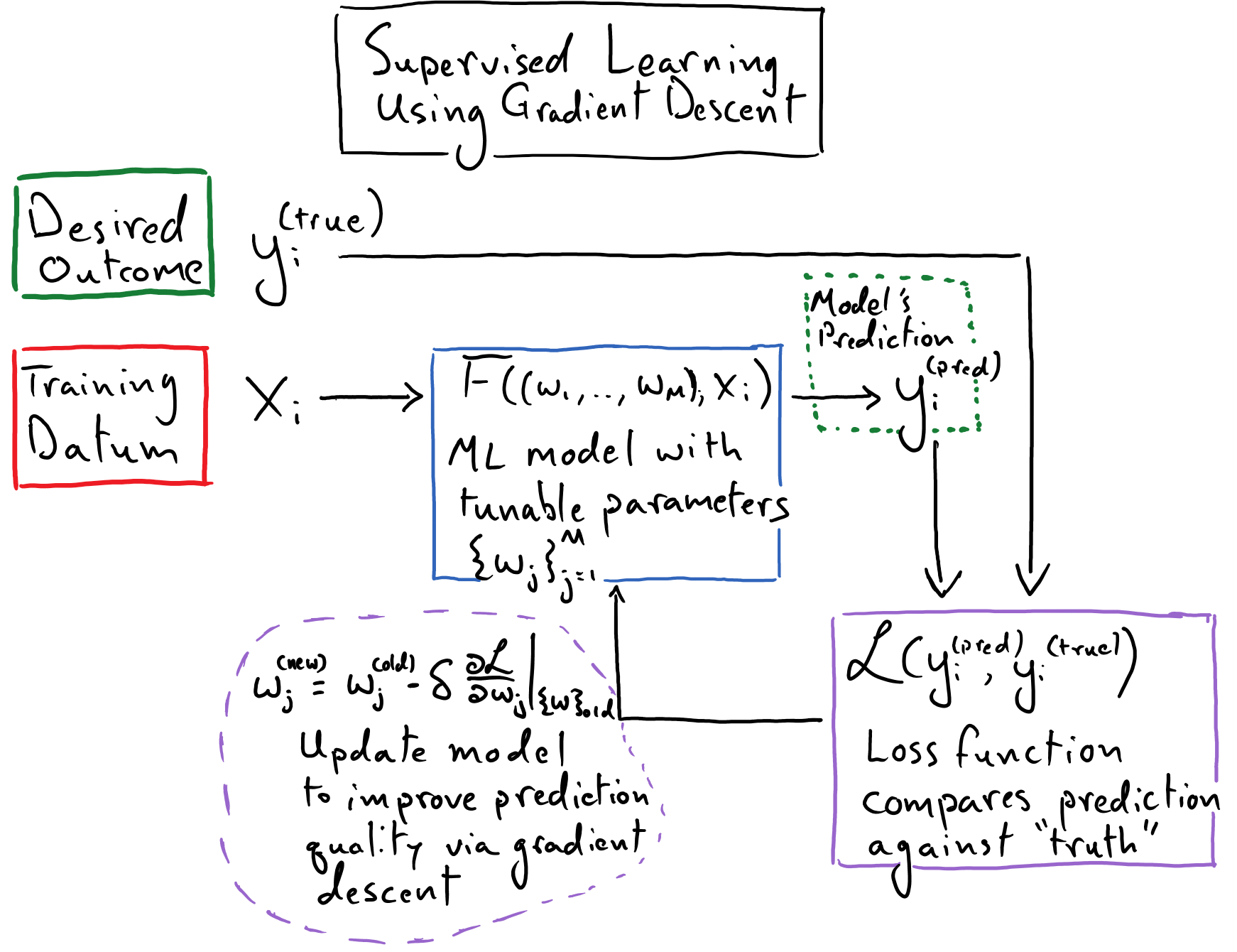
A diagram detailing the supervised learning framework

We must keep in mind our overarching objective here: given some piece of observed data, we want to arrive at some mathematical model (that is inevitably implemented as a computer program) that can produce a useful prediction or decision based on that piece of observed data. The process of learning involves tuning the numerical parameters of our model so that it produces reliable predictions or decisions when it encounters new pieces of observed data. This tuning process is frequently described as training one’s model.

The Data

In the context of supervised learning, we will need access to a dataset consisting of representative pieces of observed data along with the desired predictions or decisions that we would like our model to make when it encounters these pieces of data. Such a collection of observed data and associated desired outputs (or “truth data”, to be succinct) is used to form training, validation, and testing datasets, which, respectively, are used to modify the model’s parameters directly, to help refine the hyperparameters that we use to train the model, and to give us an ultimate quantitative measure of how well we expect our model to perform when it encounters brand-new pieces of observed data.

In our worked example, we had access to measured heights and wingspans of rookie NBA players and this served as our training data (we did not go through the process of validation or testing for this preliminary example). The heights served as pieces of observed data, and the recorded wingspans is the associated “truth data”, which, roughly speaking, are the values that we want our model to produce in correspondence with the heights. If we were interested in developing a mathematical model that can classify images (e.g. an example of a two-class image classification problem is: given the pixels of this image decide whether the picture contains a cat or a dog), then our data set would consist of images that we have collected along with associated labels for the images; the labels are the “truth data” which detail what class – dog or cat – each image belongs to.

The Model

Our model is the thing that mediates the transformation of a piece of observed data to a prediction or decision; in this way, it is the “intelligent” part of this framework. While in practice the model inevitably takes form as an algorithm implemented by a computer program, it is most useful to just think of it as a mathematical function

F ((w_{1}, \dots, w_{M}); x) = y^{(pred)}

where $F$ is the function that transforms an observation ( $x$ ) to an output ( $y^{(pred)}$ ), and $(w_{j})_{j = 1}^{M}$ is the collection of tunable parameters associated with this function. Recall that our goal is to find a numerical value for each of these $M$ parameters so that our model will make reliable predictions or decisions when it encounters new data. Let’s represent a collection of such “optimal” parameter values as $(w_{j}^{*})_{j = 1}^{M}$ , then $F ((w_{1}^{*}, \dots, w_{M}^{*}); x)$ represents our trained model.

In the context of predicting a NBA player’s wingspan based only on his height, we used the simple linear model:

F ((w_{1}, w_{2}); x) = w_{2} x + w_{1}

And once we found satisfactory values for the slope ( $w_{2}^{*}$ ) and y-intercept ( $w_{1}^{*}$ ) that produced a line closely fit our training data, we had arrived at our “trained” linear model.

But how do we write down a sensible form for $F ((w_{1}, \dots, w_{M}); x)$ when we can’t simply plot our data and plainly identify patterns shared between the inputs and outputs? In the aforementioned image classification problem, $x$ is the pixels of an image, and $F$ needs to process those pixels and return a numerical score that represents some measure of “dog-ness” or “cat-ness” for that image… I don’t know about you, but it is not obvious to me how I would write down $F$ for this problem! This is what we will refer to as the modeling problem.

Looking Ahead:

We will discuss the modeling problem further in the next section. This is where we will be introduced to the notion of a so-called “neural network”, which is a specific variety of model, $F$ , which can be used to tackle a wide variety of machine learning problems.

The Supervisor

The supervisor is responsible for comparing our model’s prediction against the “true” prediction and providing a correction to the model’s parameters in order to incrementally improve the quality of its prediction. In this course, we will inevitably create a loss function, $L (y^{(pred)}, y^{(true)})$ , that is responsible for measuring the quality of our model’s predictions. We design this to be a continuous function that compares a prediction against the “true” result and returns a value that gets smaller as the agreement between the prediction and the “truth” improves. Thus, as we saw before, we want to find the model parameters such that the average loss – taken over all $N$ pieces of data in our dataset – is minimized:

\frac{1}{N} \sum_{n = 0}^{N - 1} L (F ((w_{1}, \dots, w_{M}); x_{n}), y_{n}^{(true)})

This objective follows the empirical risk minimization principle, which posits that the ideal model parameter values, $(w_{j}^{*})_{j = 1}^{M}$ , are those that minimize the number of mistakes that our model makes across our available training data.

In our linear regression example, we used the mean squared-error as our loss function, and we searched for the optimal model parameter values, $(w_{1}^{*}, \dots, w_{M}^{*})$ , using gradient descent. Recall that we leverage automatic differentiation through both the loss function and our model in order to “measure” each $\frac{d L}{d w_{i}}$ , which we then use to update our model’s parameters via the update equation $w_{i}^{new} = w_{i}^{old} - δ \frac{d L}{d w_{i}}$ . While gradient descent is a very popular algorithm to use to optimize one’s model parameters within the supervised learning framework, it is not a required component of supervised learning: the definition of supervised learning is agnostic to the details of how one updates their model’s parameter values.

Training on Batches of Data:

The diagram above shows us feeding the model a single piece of training data, and updating the model based on the output associated with that datum. In practice, we will often feed the model a “batch” of data – consisting of $n$ pieces of input data, where $n$ is the “batch size” – and it will process each piece of data in the batch independently, producing $n$ corresponding outputs. It is also common to assemble this batch by drawing the examples at random from our pool of training data. Our loss function will then measure the quality of the model’s $n$ predictions averaged over the batch of predictions. Thus the gradient-based updates made to our model’s weights will be informed not by a single prediction but by an ensemble of $n$ predictions.

This has multiple benefits. First and foremost, by using a batch of data that has been randomly sampled from our dataset, we will find ourselves with gradients that more consistently (and “smoothly”) move our model’s weights towards an optimum configuration. The gradients associated with two different pieces of training data might vary significantly from each other, and thus could lead to a “noisy” or highly tumultuous sequence of updates to our model’s weights were we to use a batch of size $1$ . This issue is mitigated if the gradient is instead derived from a loss averaged over multiple pieces of data, where the “noisy” components of the gradient are able to cancel each other out in the aggregate and thus the gradient can more reliably steer us down the loss landscape.

Second, there are often times computational benefits to processing batches of data. For languages like Python, it is critical to be able to leverage vectorization through libraries like PyTorch and NumPy, in order to efficiently perform numerical processing. Batched processing naturally enables vectorized processing.

A final, but important note on terminology: the phrase “stochastic gradient descent” is often used to refer to this style of batched processing to drive gradient-based supervised learning. “Stochastic” is a fancy way of saying “random”, and it is alluding to the process of building up a batch of data by randomly sampling from one’s training data, rather than constructing the same batches in an ordered way throughout training.

Reading Comprehension: Filling Out the Supervised Learning Diagram

Reflect, once again, on the height-versus-wingspan modeling problem that we tackled. Step through the supervised learning diagram above, and fill out the various abstract labels with the particulars of that toy problem.

What is..

$x_{i}$
$y_{i}^{(true)}$
$F ((w_{1}, \dots, w_{M}); x)$
$y_{i}^{(pred)}$
$L (y^{(pred)}, y^{(true)})$
And how did we access each $\frac{d L}{d w_{i}}$ to form the gradient, to update our model? Did we write these derivatives out by hand?

Is Linear Regression an Example of Machine Learning?

The colloquial use of the word “learning” is wrapped tightly in the human experience. To use it in the context of machine learning might make us think of a computer querying a digital library for new information, or perhaps of conducting simulated experiments to inform and test hypotheses. Compared to these things, gradient descent hardly looks like it facilitates “learning” in machines. Indeed, it is simply a rote algorithm for numerical optimization after all. This is where we encounter a challenging issue with semantics; phrases like “machine learning” and “artificial intelligence” are not necessarily well-defined, and the way that they are used in the parlance among present-day researchers and practitioners may not jive with the intuition that science fiction authors created for us.

There is plenty to discuss here, but let’s at least appreciate the ways that we can, in good faith, view gradient descent as a means of learning. The context laid out in the preceding sections describes a way for a machine to “locate” model parameter values that minimize a loss function that depends on some observed data, thereby maximizing the quality of predictions that the model makes about said data in an automated way. In this way the model’s parameter values are being informed by this observed data. Insofar as these observations augment the model’s ability to make reliable predictions or decisions about new data, we can sensibly say that the model has “learned” from the data.

Despite this tidy explanation, plenty of people would squint incredulously at the suggestion that linear regression, driven by gradient descent, is an example of machine learning. After all, the humans were the ones responsible for curating the data, analyzing it, for deciding that the model should take on a linear form, and for using the gradient-descent algorithm to update the parameters of that linear model. Fair enough; it might be a stretch to deem this “machine learning”. But we will soon see that merely swapping out our linear model for a much more flexible (or “universal”) mathematical model will change this perception greatly. This will occur when we set out to use machine learning to tackle much more diverse and ambitious problems; in such circumstances, we will leverage mathematical models whose fundamental “shapes” are not obvious to us.

When we don’t know what the fundamental shape of our mathematical model is, the supervised learning cycle can be seen as “sculpting” an otherwise formless mathematical model, and thus informing the patterns that the model extracts and processes, based on the training data that we are using. Thus, because the data is informing the fundamental shape of the mathematical model, people feel comfortable with calling gradient-based optimization in a supervised setting “learning”. The point here is that the distinction between tuning the parameters of a linear model and “learning” the shape of a mathematical function is more subtle than one would expect. Thus, in using gradient descent to perform linear regression we have already witnessed “machine learning” to a certain extent.

Reading Comprehension Exercise Solutions

Filling Out the Supervised Learning Diagram: Solution

$x_{i}$ : is a height from our training data. I.e. it is the height of one of the players from our dataset.
$y_{i}^{(true)}$ : is the corresponding wingspan that we measured for that same player; it is what we would like our model to predict.
$F ((w_{1}, \dots, w_{M}); x)$ : is out linear model $w_{2} x + w_{1}$
$y_{i}^{(pred)}$ : is $w_{2} x_{i} + w_{1}$ , which is the predicted wingspan that our model produced based on the current values of its parameters $w_{1}$ and $w_{2}$ .
$L (y^{(pred)}, y^{(true)})$ is the mean-squared error, which we use to measure the discrepancy between our predicted wingspan and the true wingspan

L_{MSE} = \frac{1}{N} \sum_{n = 0}^{N - 1} (y_{n}^{(true)} - y_{n}^{(pred)})^{2}

We gained access to each $\frac{d L}{d w_{i}}$ (in order to perform gradient descent) by leveraging the automatic differentiation library MyGrad.