Word Embeddings and Autoencoders

So far, we have experimented with the bag-of-words approach to analyze documents and determine their similarity to other documents. This is a good starting point for understanding the contents of a document, but falls short on two accounts: it fails to consider word order and synonyms.

1. ignores word order

Say we have doc1 = "the boy gave the book to the girl" and doc2 = "the girl gave the book to the boy".

	boy	book	gave	girl
doc1	\(1\)	\(1\)	\(1\)	\(1\)
doc2	\(1\)	\(1\)	\(1\)	\(1\)

doc1 and doc2 appear totally identical!

2. ignores synonyms

Say we have doc1 = "the woman was happy" and doc2 = "the lady was glad".

	glad	happy	lady	woman
doc1	\(0\)	\(1\)	\(0\)	\(1\)
doc2	\(1\)	\(0\)	\(1\)	\(0\)

doc1 and doc2 appear totally different!

In this lecture, we’re going to be exploring a very important building block for representing text called “word embeddings”.

Introduction to Word Embeddings

Word embeddings are a technique for mapping discrete words to a continuous space.

• e.g., “happy” –> [0.2, -0.3] maps the word “happy” in a 2-dimensional space

Creating embeddings for words is a more desirable way to process language than the bag-of-words approach because

1. Using word embeddings can help with synonym problem (since techniques for learning word embeddings tend to map similar words to similar embeddings)

   • e.g., “glad” –> [0.19, -0.32]

2. Models can have fewer parameters

For example, suppose we wanted to use a simple NN for language modeling that predicts the next word given the previous two. As we know from working with neural networks in past weeks, we must find have some numerical representation of each word that we pass into it. One way we can do this is with one-hot encodings. A one-hot encoding is a vector of dimension \(n\) where there are \(n\) words in your vocabulary. A vocabulary is simply the set of all words in all the documents you are considering. The one-hot encoding for a word is comprised of all zeros except for 1 in slot corresponding to the word. inputs would be size 2 * |vocab| since each of the two previous words is represented by a vector of size |vocab|.

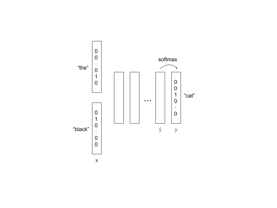
This becomes an issue because the vocabulary you are working with can often have tens of thousands to hundreds of thousands of words in it.

If we instead rely on word embeddings as our input, we can have a constant input size regardless of the vocabulary size. For example, if we use word embeddings of dimension 50 (mapping each word in a 50-dimensional space), our input size will be 100 regardless of the size of our vocabulary. Recall that we saw a similar idea during the computer vision capstone project when we used face descriptor vectors to represent a face. Similar faces should have similar face descriptors, or embeddings. This week, we will rely on word embeddings to represent a word, and thus similar words should have similar embeddings.

Introduction to Autoencoders

In cogworks, we try to demystify everything and do as much from scratch as possible, so we’d like to look at a way to perform a dimensionality reduction with a model called an “autoencoder”. An autoencoder is a type of neural network that aims to “learn” how to represent input data in a dimensionally reduced form. The neural network is essentially trained to focus on the most important “features” of input data to find an encoding that effectively distinguishes it from other input data while reducing dimensionality.

We will see that autoencoders prove helpful in reducing the dimension of word embeddings via unsupervised learning…

Training Your Own Word Embeddings: Unsupervised Learning

Now that we know what word embeddings and autoencoders are, we can begin exploring how to compute our own embeddings. First, let’s talk about supervised vs unsupervised learning. Supervised learning involves training a model where there are known “answers” or truth values for each data point. In other words, there are input-output pairs so we can directly assess whether or not our model produced the correct answer. The work you did with the CIFAR-10 dataset during the Audio module involved supervised learning because each image had a label.

Unsupervised learning involves training a model where there is not “answer” or truth value. This is often visualized as clustering data in a continuous space without being provided any labels. For example, a model that takes in student profiles may produce clusters that contain athletes, musicians, artists, etc. without having been provided any actual labels. In general, we turn to unsupervised learning when we want to find similarities among our data, but there is no concrete value we want to achieve. Unsupervised learning is great because the data is cheaper and easier to collect since we don’t need to label each data point with a truth value, like how someone had to label each image CIFAR-10.

As you may have guessed, many word embedding techniques rely on unsupervised learning to cluster words in continuous space based on their context to each other. Unsupervised learning proves to be very convenient for embedding words because there is a large amount of existing text out there and we don’t need to add target labels.

Note: technically this is an example of “self-supervised” learning because the target labels (embeddings) are automatically extracted from the data itself. To achieve dimensionality reduction in our word embeddings via an autoencoder, we will utilize a loss function that essentially compares the inputted embedding to the outputted/recovered embedding according to the following equation

\begin{equation} L(x_\text{recovered},x_\text{original}) = \frac{1}{N} \sum_{i=0}^{N-1} (x_\text{recovered} - x_\text{original})^2 \end{equation}

Thus, we are utilizing self-supervised learning to extract “truth values” from the data itself in order to train our autoencoder to produce effective word embeddings.

Approaches to Training Word Embeddings

There are many interesting approaches for training word embeddings. Many rely on the idea that words that appear in similar contexts are similar. Let’s cover a few different methods for training word embeddings

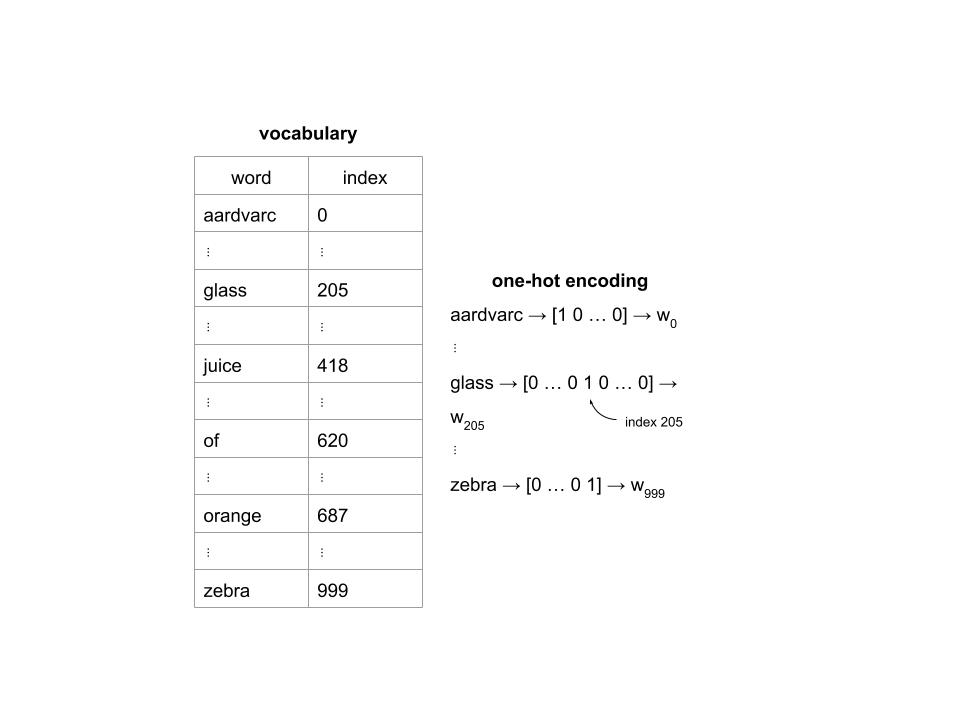
One-hot encoding, as we mentioned earlier, is a very simple way to create word embeddings based on a vocabulary of \(n\) words. Each word is represented by an \(n\)-dimensional vector of zeros with a single \(1\) in the alphabetical location corresponding to the word. Say we have a vocabulary of \(1000\) words and the phrase “glass of orange juice” We can form the one-hot encodings as follows

We can use one-hot encodings to help us (1) predict the next word given a history of words, (2) predict the middle word given the context words to the left and right, and (3) predict the context words given a word in the middle.

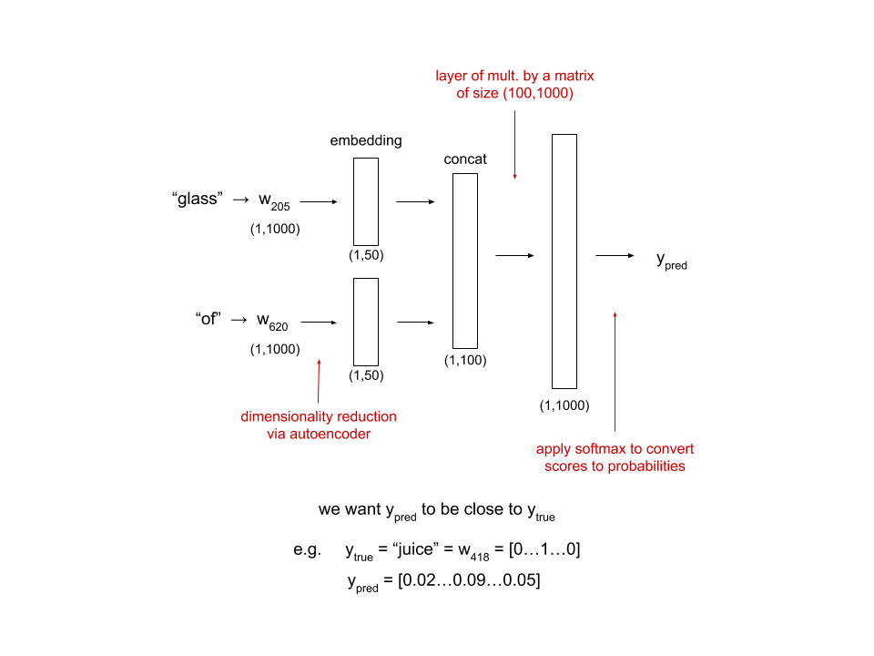
Say we have a history “glass of” and want to predict the next word. Recall that we are working with a vocabulary of 1000 words.

Now, say we want to use a target word to predict the context words. This is done using an unsupervised learning technique called a skip-gram, which takes the target word as an input and outputs context words. Given the target word “orange”, the probabilities of the skip-gram producing various words as contextually related are as follows

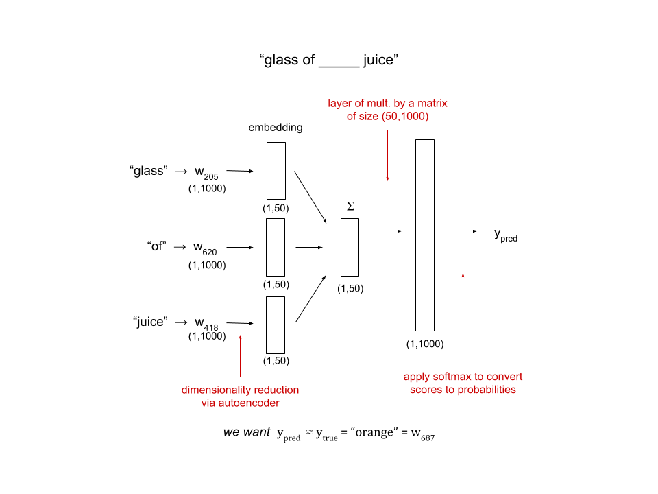
Finally, say we want to use the context words to predict the word in middle. This is done using a method called CBOW (Common Bag of Words), which takes context words as input and outputs the target word. Given the context words “glass”, “of”, and “juice”, our neural network will look like

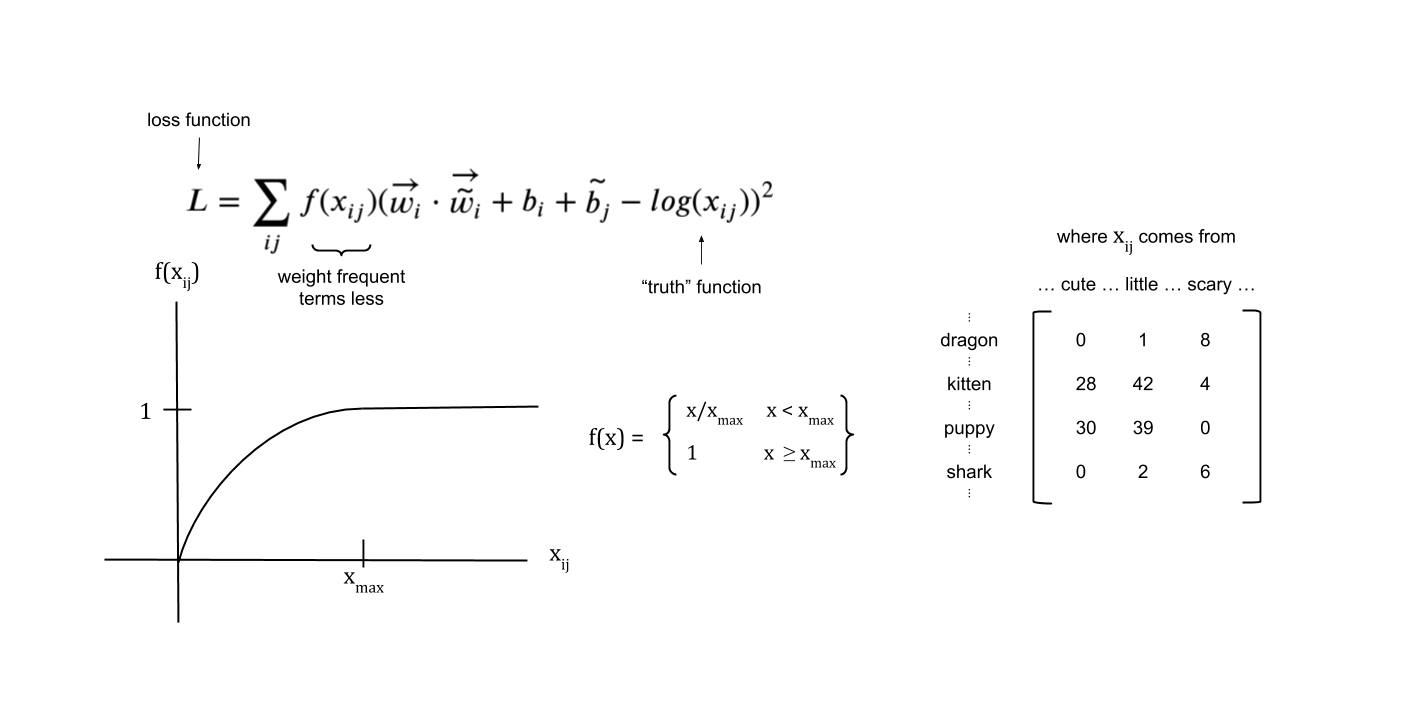
One final method is to create embeddings by mapping words to a continuous space based on their “semantic similarity” or the similarity of their meanings. This is done by directly modeling \(X_{ij}\) (the number of times word \(j\) occurs in the context of word \(i\)). Essentially, the dot product of \(w_i\) and \(w_j\) (plus biases) approximates \(log(X_{ij})\). The bias terms are vectors that we initialize with a normal distribution to help achieve the best fit as a model is training. This has already been done via unsupervised learning techniques and is known as the Global Vectors for Word Representation (GloVe).

We’re going to employ the concept of an autoencoder to do a dimensionality reduction on a global matrix of words by contexts. By reducing the dimension of the GloVe embeddings, the autoencoder effectively distills critical relational features, making the embeddings more concise.

Sentiment Analysis

didn’t do in 2019?

Now that we know where word embeddings come from, what can we use them for?

• language modeling

• representing/encoding documents

• averaging word embeddings of words in a sentence is an option

  • but not great since ignores word order

• can use CNN, RNNs