Language Module Capstone: Semantic Image Search

Now that we’re familiar with different methods for understanding language through word embeddings, let’s apply these skills to semantically search a database of images based on a natural language query. That is, given the user-provided query “horses on a beach” we want to find images of horses on a beach based solely on the appearances of those images. A user can ostensibly type in any query, and we will try to look for images that resemble the query’s description.

This project will bring together different concepts we’ve covered in this course, including word embeddings, image embeddings (descriptors), and encoders. We’ve seen many examples of embeddings, or vectors meant to describe an object, throughout the course. These include GloVe word embeddings, FaceNet facial descriptors, and bag of words vectors. The common theme for these embeddings is that similar objects (synonymous words or images of the same face from different angles) have similar embeddings (this can be determined using cosine similarity).

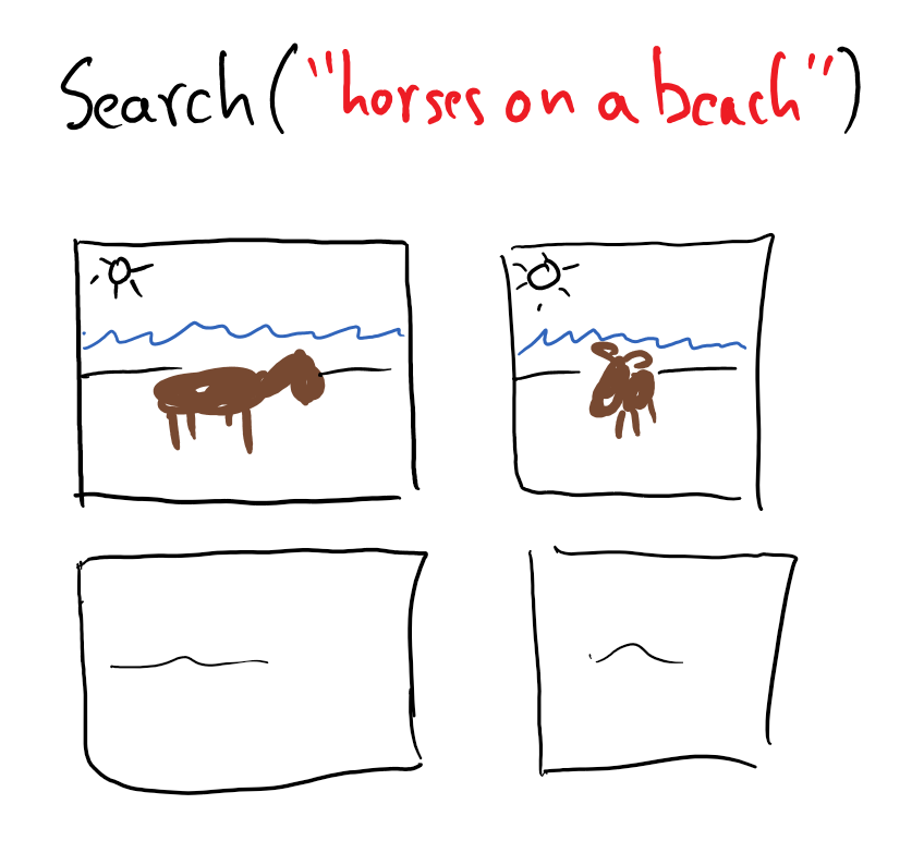
In order to semantically search through a database of images, we’re going to apply this same concept but across different object types. Namely, we want to find images that are semantically similar to words. Instead of relying on embeddings in the word space to find similar words or the face space to find similar faces, we are going to search the semantic space to find images that are similar to words.

Let’s break this down into the following pieces

Overview of the project

What data do we have access to?

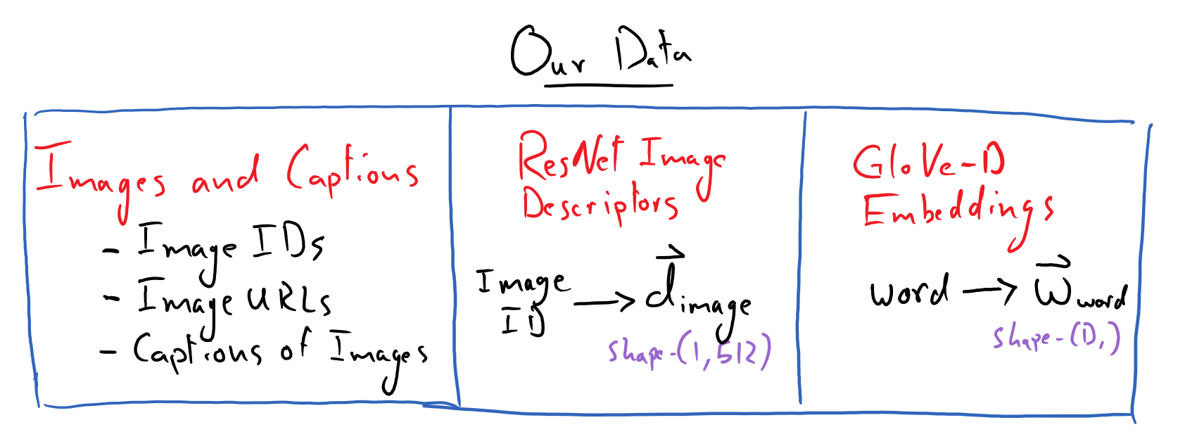
We will be given a large dataset – MSCOCO 2014 – of curated images, where each image has multiple captions associated with it that describes that image. Note that this dataset is so large that we will not actually download the images, but will have access to a URL for each image, where we can download that image if need-be. - Each image will have an associated unique ID - Each caption will also have a unique ID. - One image can have multiple captions associated with it, but each caption is only associated with a .single image.

We will also be given access to pre-computed descriptor vectors for all of the images. Each image has one shape-\((512,)\) descriptor vector. These are just like word-embeddings, but for images. These were computed using a trained ResNet model that is excellent at image classification tasks. Thus a descriptor vector for an image is a condensed, abstract representation of the semantic contents of that image. E.g. a pair of pictures of red cars on highways will have corresponding descriptor vectors that are similar to one another (as measured by the dot product).

Lastly, we will have access to GloVe word embedding vectors. We will use the \(D=200\)-dimensional vectors. These will be used to create embedding vectors for both image captions and for queries, such that a query/caption will also have a shape-\((200,)\) embedding vector representation. More on this later.

Here is a picture to summarize our data:

How do we make embeddings for captions and queries?

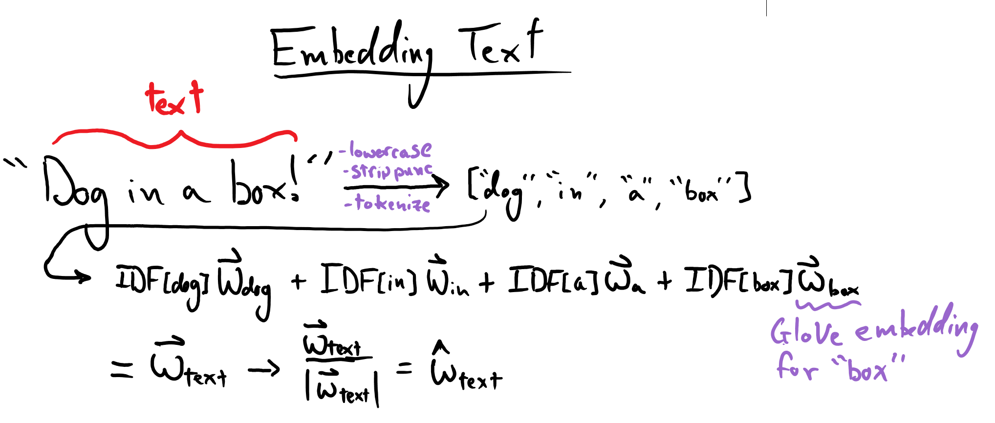
Each caption’s/query’s embedding will be formed using a weighted sum of the GloVe embedding for each word in the caption/query. The weight for a given word will be given by the inverse document frequency (IDF) for that word. Note that we will lowercase all queries & captions, strip punctuation out of them, and tokenize them, but we will retain stop words (a.k.a glue words) in them. Note that the inverse document frequency for a word is computed across all captions in our dataset (i.e. each caption counts as its own “document”).

If a query involves a word that is not found among our captions, we will say that its IDF is 0.

Here is a picture that describes this process:

How do we make use of our image descriptor and word embeddings?

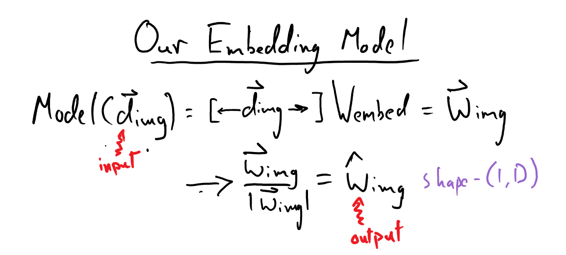
As mentioned before, we want to be able to represent each image, based on its appearance, in the same semantic space as the words in our captions/queries. To achieve this, we will train a simple linear encoder that will map each image’s shape-\((1, 512)\) descriptor (\(\vec{d}_{\mathrm{img}}\)) vector to a shape-\((1, 200)\) embedding vector (\(\vec{w}_{\mathrm{img}}\)):

\begin{equation} \vec{d}_{\mathrm{img}} W_{\mathrm{embed}} = \vec{w}_{\mathrm{img}} \end{equation}

\begin{equation} \hat{w}_{\mathrm{img}} = \frac{\vec{w}_{\mathrm{img}}}{||\vec{w}_{\mathrm{img}}||} \end{equation}

(we will want to work with normalized embedding vectors for all of our images, captions, and queries throughout this project).

Fitting our linear embedding matrix

How do we find \(W_{\mathrm{embed}}\) such that \(\hat{w}_{\mathrm{img}}\) faithfully represents information about our image, but in the shared semantic space with our caption embeddings?

We will “train” (fit) \(W_{\mathrm{embed}}\) using a triplet loss that encourages an image’s embedding vector to be similar to the embedding vectors for its captions. Specifically, we will pick an image and one of its captions; we will call this the “true” image. Then we will pick a “confusor” image.

Using \(W_{\mathrm{embed}}\) (whose values we are refining via this training process), we will compute \(\hat{w}^{\mathrm{true}}_{\mathrm{img}}\) and \(\hat{w}^{\mathrm{confusor}}_{\mathrm{img}}\). Then we will use a loss function that enforces: \(\hat{w}^{\mathrm{true}}_{\mathrm{img}} \cdot \hat{w}_{\mathrm{caption}} > \hat{w}^{\mathrm{confusor}}_{\mathrm{img}} \cdot \hat{w}_{\mathrm{caption}}\).

The loss function that we will use is known as the margin ranking loss. MyGrad has an implementation of it.

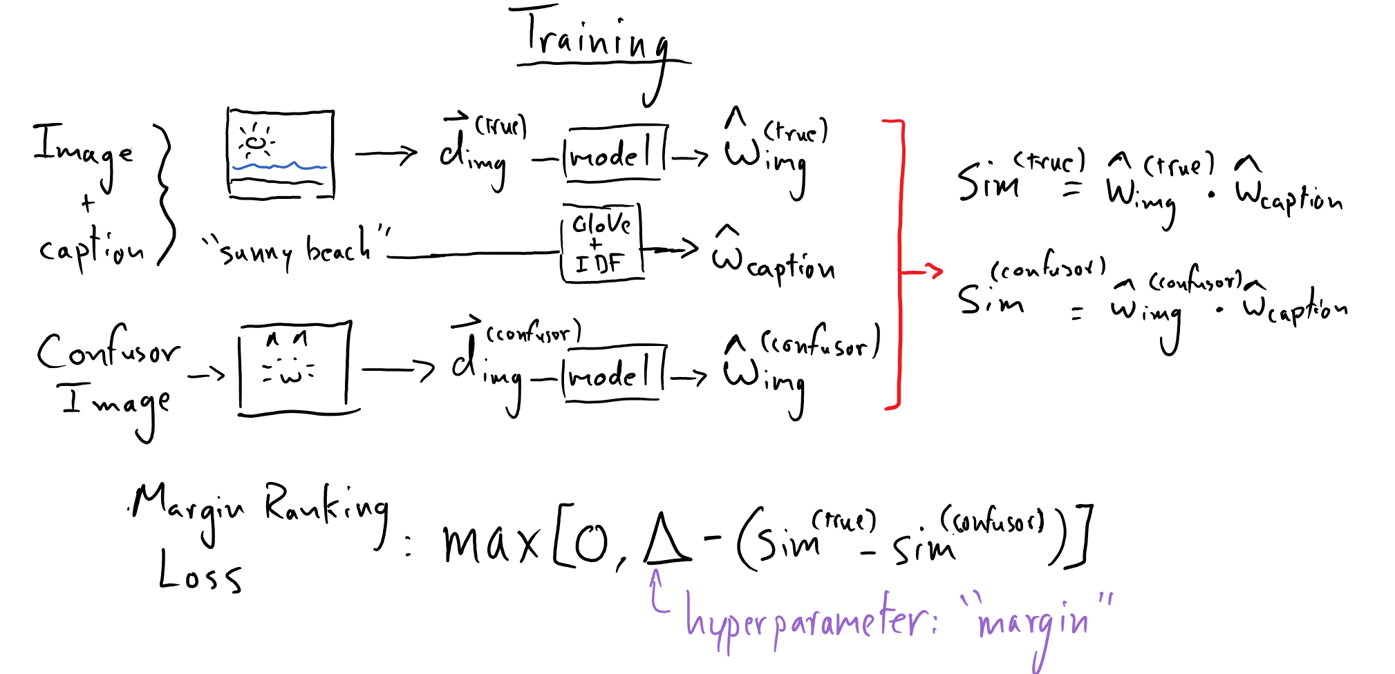
Once we fit \(W_{\mathrm{embed}}\) we will be able to describe all of our images in a common semantic space, shared with the embeddings for captions and queries!

What is our database of images and how do we search images with a query

The images that we can store in our database are those for which we have a shape-\((512,)\) descriptor vector. Thus we can store all of the images from the COCO 2014 dataset. We will use \(W_{\mathrm{embed}}\) to compute \(\hat{w}_{\mathrm{img}}\) for each of those images and simply store those in a shape-\((N, 200)\) array (where \(N\) is the total number of images we have).

Whenever we get in a new query, we convert that text to an embedding vector – using the GloVe & IDF method from above – and then compute the dot product between it and all of our \(N\) of our image embedding vectors. This will produce \(N\) similarity scores – the top-\(k\) scores will indicate the \(k\) most relevant images, which we can download and display to the user (more on this later).

Here is a picture that describes this:

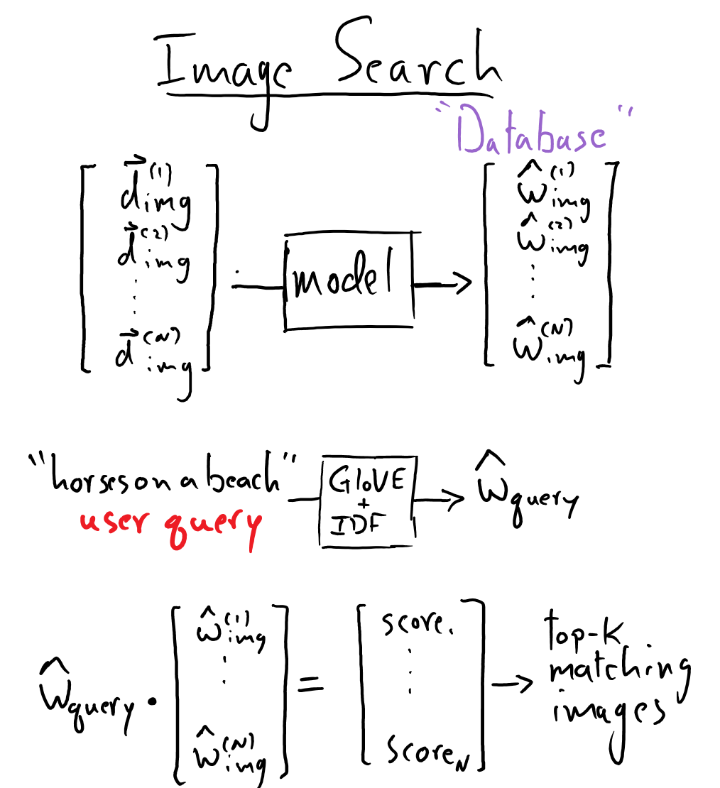
To summarize the above..

Image-descriptor vectors (which have already been processed for us) will be denoted by \(\vec{d}\) (shape-\((512,)\)). Vectors in the embedded language space will be denoted by \(\vec{w}\) (shape-\((200,)\)). A vector denoted with a “hat” – \(\hat{w}\) – indicates a normalized vector.

We want to learn the following linear encoding:

\begin{align} &\begin{bmatrix}\leftarrow & \vec{d}_{\mathrm{image}} & \rightarrow \end{bmatrix} W_{\mathrm{embed}} = \begin{bmatrix}\leftarrow & \vec{w}_{\mathrm{image}} & \rightarrow \end{bmatrix} \end{align}

where \(\vec{d}_{\mathrm{image}}\) is a \(512\)-dimensional descriptor vector of an image, produced by a pre-trained ResNet-18 image-classification model. \(\vec{w}_{\mathrm{image}}\) is a \(D=200\)-dimensional embedding of this image descriptor. We want this embedded vector to “live” in the same “semantic space” as word embeddings.

Suppose we want to search for pictures of “horses on a beach”. We can use the \(D\)-dimensional GloVe embedding for each word in this “caption”, and sum these word-embeddings with weights determined by the inverse document frequency (IDF) of each word (we will discuss how these IDFs get computed later). Thus we can form the embedding for this caption as:

\begin{equation} \mathrm{IDF(\mathrm{horses}})\vec{w}_{\mathrm{horses}} + \mathrm{IDF(\mathrm{on}})\vec{w}_{\mathrm{on}} + \mathrm{IDF(\mathrm{a}})\vec{w}_{\mathrm{a}} + \mathrm{IDF(\mathrm{beach}})\vec{w}_{\mathrm{beach}} = \vec{w}_{\mathrm{caption}} \end{equation}

where \(\vec{w}_{\mathrm{horses}}\) is the \(D\)-dimensional GloVe embedding vector for the word “horses”, and \(\mathrm{IDF(\mathrm{horses}})\) is the inverse document-frequency for “horses” (a positive scalar quantity).

If we have a picture depicting horses on a beach and its corresponding descriptor vector, \(\vec{d}_{\mathrm{image}}\) (which we are given – these image descriptor vectors have been pre-created for us), then we want to be able to embed the descriptor vector for that image to some \(\vec{w}_{\mathrm{image}}\), such that an embedding vector for the caption, \(\vec{w}_{\mathrm{caption}}\), overlaps substantially with the image’s embedding.

\begin{equation} \vec{d}_{\mathrm{\mathrm{image}}}W_{\mathrm{embed}} \rightarrow \vec{w}_{\mathrm{image}}\\ \end{equation} \begin{equation} \hat{w}_{\mathrm{image}}\cdot \hat{w}_{\mathrm{caption}} >> 0\\ \end{equation}

We can use these similarity scores to look for good matches between a query and images.

Our Data

Downloading the Data

There are three datasets that we need:

• The GloVe word embeddings for a broad vocabulary of words.

  • (you don’t need to download this manually, we will provide convenience functions) glove.6B.200d.txt.w2v.zip (258 MB)

• Captions that describe images from the MSCOCO dataset, and URLs for fetching those images.

  • (you don’t need to download this manually, we will provide convenience functions) MS COCO captions

• A descriptor vector for each image from the MSCOCO dataset, produced from a pre-trained ResNet-18 classification model. This serves as an enriched/abstract encoding for each image in the dataset.

  • (you don’t need to download this manually, we will provide convenience functions) ResNet-18 image descriptors.

We are going to be working with the MSCOCO 2014 dataset. This dataset consists of 82,783 images, and each image has at least five plain-text captions that describe that image. These images have also been processed using a pre-trained ResNet-18 classification model, such that we also have a \(512\)-dimensional descriptor vector, \(\vec{d}_{\mathrm{\mathrm{image}}}\), associated with each image, which captures the contents of that image in an abstract way.

All of the pertinent data for this project is found in three data file:

1. Images and associated captions from the MSCOCO 2014 dataset. All of this information is stored in the captions_train2014.json JSON file. A few notes about this:

   • We won’t download all of the images at once, rather we will have a URL that we can use to download any given image.

   • Each image has associated with it at least one, but possibly more, plain-text captions that describe it.

2. A shape-\((1, 512)\) descriptor vector, \(\vec{d}_{\mathrm{\mathrm{image}}}\), for each image from the MSCOCO dataset. Each of these was produced by processing each image with a pre-trained ResNet-18 classification model. This serves as an enriched/abstract encoding for each image in the dataset. resnet18_features.pkl contains a dictionary of image-ID -> descriptor-vector mappings, where image-ID is a unique integer ID for each image in the COCO-dataset. There are three files that we need for this project:

3. The GloVe-200 word embeddings for a broad vocabulary of words. This will be used to compute \(D=200\)-dimensional embedding vectors \(\hat{w}_{\mathrm{caption}}\) for each caption. These are stored in "glove.6B.200d.txt.w2v"

Loading COCO Data

from cogworks_data.language import get_data_path

from pathlib import Path
import json

# load COCO metadata
filename = get_data_path("captions_train2014.json")
with Path(filename).open() as f:
    coco_data = json.load(f)

>>> len(coco_data["images"])  # number of images
82783

>>> coco_data["images"][0]
{'license': 5,
 'file_name': 'COCO_train2014_000000057870.jpg',
 'coco_url': 'http://images.cocodataset.org/train2014/COCO_train2014_000000057870.jpg',
 'height': 480,
 'width': 640,
 'date_captured': '2013-11-14 16:28:13',
 'flickr_url': 'http://farm4.staticflickr.com/3153/2970773875_164f0c0b83_z.jpg',
 'id': 57870}

The "captions_train2014.json" JSON file has two fields that we care about: “images” and “annotations”.

coco_data["images"] contains a list; each entry corresponds to a distinct image. For example image_info = coco_data["images"][0] stores information for the first image. Each such entry contains:

• A unique integer ID for the image (image_info["id"])

• The URL where you can download the image (image_info["coco_url"])

• The shape of the image (image_info["height"], image_info["width"])

coco_data["annotations"] contains a list; each entry corresponds to a distinct caption. For example caption_info = coco_data["annotations"][0] stores information for the first caption. Each such entry contains:

• A unique integer ID for the caption (caption_info["id"])

• The ID of the image that this caption is associated with (caption_info["image_id"])

• The caption, stored as a string (caption_info["caption"])

>>> len(coco_data["annotations"])  # number of captions
414113

>>> coco_data["annotations"][0]
{'image_id': 318556,
 'id': 48,
 'caption': 'A very clean and well decorated empty bathroom'}

Keep in mind that there are multiple captions associated with each image. Thus there are 82,783 entries to coco_data["images"] and 414,113 entries to coco_data["annotations"].

Loading GloVe Embedding and Creating Embeddings of Our Captions

First, we will load the GloVe-200 embeddings:

from gensim.models import KeyedVectors
filename = "glove.6B.200d.txt.w2v"

# this takes a while to load -- keep this in mind when designing your capstone project
glove = KeyedVectors.load_word2vec_format(get_data_path(filename), binary=False)

>>> glove["apple"]
array([-0.11359  ,  0.20144  , -0.47074  , -0.028013 ,  0.67625  ,
       -1.0141   , -0.29246  , -0.28873  ,  0.13012  ,  0.31178  ,
      ...
      ...
        0.12729  , -0.38416  ,  0.24395  , -0.18857  ,  0.4942   ,
       -0.14013  , -0.39927  , -0.42846  ,  0.37869  , -0.52865  ],
      dtype=float32)

>>> glove["apple"].shape  # a shape-(200,) word embedding

>>> glove["apple"] @ glove["pear"]  # (un-normalized) dot-produce of apple and pear
20.519402

>>> glove["apple"] @ glove["truck"]  # (un-normalized) dot-produce of apple and truck
4.623803

Because we have access all of the captions associated with the COCO images, we can compute a single embedding vector for each of our captions. Some notes on processing captions:

• We will lowercase, remove punctuation, and tokenize any caption that we work with.

• We will not worry about removing stop (a.k.a glue) words from our captions.

We compute the inverse document frequency (IDF) of every term that appears in the captions, across all captions

\begin{equation} \mathrm{IDF(t)} = \log_{10}{\frac{N_{\mathrm{captions}}}{n_{t}}} \end{equation}

where \(n_{t}\) is the number of captions that term-\(t\) appears in, and \(N_{\mathrm{captions}}\) is the total number of captions.

Each caption’s embedding is created via an IDF-weighted sum of the glove-embedding for each word in the caption. We then normalize this vector E.g, if the caption was “Horses on a beach”, then the following shape-(\(D=200\),) embedding would be formed via:

\begin{equation} \mathrm{IDF(\mathrm{horses}})\vec{w}_{\mathrm{horses}} + \mathrm{IDF(\mathrm{on}})\vec{w}_{\mathrm{on}} + \mathrm{IDF(\mathrm{a}})\vec{w}_{\mathrm{a}} + \mathrm{IDF(\mathrm{beach}})\vec{w}_{\mathrm{beach}} = \vec{w}_{\mathrm{caption}} \end{equation} \begin{equation} \mathrm{norm}(\vec{w}_{\mathrm{caption}}) \rightarrow \hat{w}_{\mathrm{caption}} \end{equation}

where, e.g., \(\vec{w}_{\mathrm{horses}}\) is the \(D\)-dimensional GloVe embedding vector for the word “horses”, and \(\mathrm{IDF(\mathrm{horses}})\) is the inverse document-frequency for “horses” (a positive scalar quantity).

Loading Image Descriptor Vectors

# load saved image descriptor vectors
import pickle
with Path(get_data_path('resnet18_features.pkl')).open('rb') as f:
    resnet18_features = pickle.load(f)

resnet18_features is simply a dictionary that stores a \(\vec{d}_{\mathrm{image}}\) for each image:

image-ID -> shape-(512,) descriptor

>>> img_id = 57870
>>> resnet18_features[57870]
array([[1.04235423e+00, 6.82473838e-01, 9.16481733e-01, 2.32561696e-02,
        1.45509019e-01, 7.50707984e-01, 1.54418981e+00, 8.72745886e-02,
        2.67963076e+00, 3.70128679e+00, 2.69317198e+00, 5.91564715e-01,
        ...
        ...
        4.63250205e-02, 7.64195085e-01, 9.27642107e-01, 9.45607066e-01,
        6.30564749e-01, 7.90123463e-01, 4.79690343e-01, 6.89100996e-02,
        7.30290413e-01, 7.14914918e-01, 1.48940217e+00, 1.47434247e+00]],
      dtype=float32)

>>> resnet18_features[57870].shape
(1, 512)

where the image-IDs correspond to those in the COCO dataset.

Note that not all COCO images have ResNet descriptors associated with them:

>>> len(resnet18_features) < len(coco_data["images"])
True

>>> len(resnet18_features)
82612
>>> len(coco_data["images"])
82783

# all images in the `resnet18_features` are present among the coco images
>>> set(resnet18_features) < set(img["id"] for img in coco_data["images"])
True

thus you should discard/ignore any COCO image (and its captions) for which you do not have a ResNet descriptor.

Training Data

The basics of forming our training data is the following process:

• Separate out image IDs into distinct sets for training and validation

• Pick a random training image and one of its associated captions. We’ll call these our “true image” and “true caption”

• Pick a different image. We’ll call this our “confusor image”.

Thus our training and each validation data consist of triplets: (true-caption-ID, true-image-ID, confusor-image-ID). We will use batches of these triplets to train our model.

Training

Our Model

Our model simply consists of one matrix that maps a shape-(512,) image descriptor into a shape-(D=200,) embedded vector, and normalizes that vector.

\begin{align} &\begin{bmatrix}\leftarrow & \vec{d}_{\mathrm{image}} & \rightarrow \end{bmatrix} W_{\mathrm{embed}} = \begin{bmatrix}\leftarrow & \vec{w}_{\mathrm{image}} & \rightarrow \end{bmatrix} \\ \end{align} \begin{align} \mathrm{norm}(\vec{w}_{\mathrm{image}}) \rightarrow \hat{w}_{\mathrm{image}} \end{align}

Our Loss Function

Recall that we have formed triplets of (true-caption-ID, true-image-ID, confusor-image-ID). We will use these to form a triplet of embedding vectors. We can simply look up the embedding vector for our caption:

• true-caption-ID \(\rightarrow \hat{w}^{\mathrm{(true)}}_{\mathrm{caption}}\)

And we can retrieve the descriptor vector for both of our images

• true-image-ID \(\rightarrow \vec{d}^{\mathrm{(true)}}_{\mathrm{image}}\)

• confusor-image-ID \(\rightarrow \vec{d}^{\mathrm{(confusor)}}_{\mathrm{image}}\)

Processing these descriptors with our model will embed them in the same \(D=200\)-dimensional space as our captions:

\begin{align} \mathrm{model}(\vec{d}^{\mathrm{(true)}}_{\mathrm{image}}) &= \hat{w}^{\mathrm{(true)}}_{\mathrm{image}} \\ \mathrm{model}(\vec{d}^{\mathrm{(confusor)}}_{\mathrm{image}}) &= \hat{w}^{\mathrm{(confusor)}}_{\mathrm{image}}\\ \end{align}

We want to embed our image’s descriptor in a meaningful way, such that the contents of the image reflect the semantics of its captions. Thus we want

\begin{equation} \hat{w}^{\mathrm{(true)}}_{\mathrm{image}} \cdot \hat{w}^{\mathrm{(true)}}_{\mathrm{caption}} > \hat{w}^{\mathrm{(confusor)}}_{\mathrm{image}} \cdot \hat{w}^{\mathrm{(true)}}_{\mathrm{caption}} \end{equation}

We can enforce this using a margin ranking loss:

\begin{align} \mathrm{sim}_{\mathrm{true}} &= \hat{w}^{\mathrm{(true)}}_{\mathrm{image}} \cdot \hat{w}^{\mathrm{(true)}}_{\mathrm{caption}} \\ \mathrm{sim}_{\mathrm{confusor}} &= \hat{w}^{\mathrm{(confusor)}}_{\mathrm{image}} \cdot \hat{w}^{\mathrm{(true)}}_{\mathrm{caption}} \\ \end{align}

\begin{align} \mathscr{L}(\mathrm{sim}_{\mathrm{true}}, \mathrm{sim}_{\mathrm{confusor}}; \Delta) = \max(0, \Delta - (\mathrm{sim}_{\mathrm{true}} - \mathrm{sim}_{\mathrm{confusor}})) \end{align}

Note that all of our dot-products are involving unit vectors, thus we are computing cosine-similarities. See that this loss function encourages \(\mathrm{sim}_{\mathrm{true}}\) to be larger than \(\mathrm{sim}_{\mathrm{confusor}}\) by at least a margin of \(\Delta\).

Of course, we will be training on batches of triplets. MyGrad’s margin ranking loss will automatically compute the mean over the batch dimension. Note that einsum can be used to take pair-wise dot products across two batches of vectors. E.g. mg.einsum("nd,nd -> n", a, b) will take two shape-\((N, D)\) arrays and compute \(N\) dot products between corresponding pairs of shape-(\(D\),) vectors.

Searching Our Database

It is time to create a database of images that we can search through based on user-written queries. We will populate this database using only images from our validation set so that we know that the quality of our results isn’t from “overfitting” on our data.

We have trained our embedding matrix, \(W_{\mathrm{embed}}\), we can embed each of the image descriptors from our validation set into the caption semantic space.

\begin{align} &\begin{bmatrix}\leftarrow & \vec{d}^{(image)}_1 & \rightarrow \\ \leftarrow & \vec{d}^{(image)}_2 & \rightarrow \\ \vdots & \vdots & \vdots \\ \leftarrow & \vec{d}^{(image)}_{N_{val}} & \rightarrow\end{bmatrix} \rightarrow \mathrm{model(\dots)} \rightarrow \begin{bmatrix}\leftarrow & \hat{w}^{(image)}_1 & \rightarrow \\ \leftarrow & \hat{w}^{(image)}_2 & \rightarrow \\ \vdots & \vdots & \vdots \\ \leftarrow & \hat{w}^{(image)}_{N_{val}} & \rightarrow\end{bmatrix} \end{align}

This is our “database” of images. How do we search for relevant images given a user-supplied query? First, we embed the query in the same way that we embedded the captions (using an IDF-weighted sum of GloVe embeddings).

\begin{equation} \mathrm{"horses \; on \; a \; beach"} \rightarrow \mathrm{IDF(\mathrm{horses}})\vec{w}_{\mathrm{horses}} + \mathrm{IDF(\mathrm{on}})\vec{w}_{\mathrm{on}} + \mathrm{IDF(\mathrm{a}})\vec{w}_{\mathrm{a}} + \mathrm{IDF(\mathrm{beach}})\vec{w}_{\mathrm{beach}} \rightarrow \hat{w}_{\mathrm{query}} \end{equation}

Then we compute the dot product of this query’s embedding against all of our image embeddings in our database.

\begin{align} \begin{bmatrix}\hat{w}_{\mathrm{query}} \cdot \hat{w}^{(image)}_1 \\ \hat{w}_{\mathrm{query}} \cdot \hat{w}^{(image)}_2 \\ \vdots \\ \hat{w}_{\mathrm{query}} \cdot \hat{w}^{(image)}_{N_{val}}\end{bmatrix} \rightarrow \mathrm{top-}k\;\mathrm{similarity \; scores} \end{align}

the top-\(k\) cosine-similarities points us to the top-\(k\) most relevant images to this query! We need image-IDs associated with these matches and then we can fetch their associated URLs from our COCO data. The code for downloading an image is quite simple thanks to the PIL and requests library! Note that these images can be fetched quickly, so you need not download all of the images beforehand; you can retrieve the relevant images “on the fly” during the search process.

You can install these libraries with pip install requests pillow or conda install -c conda-forge requests pillow.

import io

import requests
from PIL import Image


def download_image(img_url: str) -> Image:
    """Fetches an image from the web.

    Parameters
    ----------
    img_url : string
        The url of the image to fetch.

    Returns
    -------
    PIL.Image
        The image."""

    response = requests.get(img_url)
    return Image.open(io.BytesIO(response.content))

Team Tasks

Below you’ll find a list of tasks that your team needs to cover to successfully complete this capstone project.

Organizing the COCO data:

• Create a class that organizes all of the COCO data. It might store the following

  • All the image IDs

  • All the caption IDs

  • Various mappings between image/caption IDs, and associating caption-IDs with captions

    • image-ID -> [cap-ID-1, cap-ID-2, ...]

    • caption-ID -> image-ID

    • caption-ID -> caption (e.g. 24 -> "two dogs on the grass")

Embedding queries and captions:

• Process captions/queries by lowercasing the text, removing punctuation, and tokenizing words based on white space. Refer to the “bag of words” exercise notebook for efficient code for striping punctuation out of a string

• Take our vocabulary to be all words across all captions in the COCO dataset. Treating each caption as its own “document” compute the inverse document frequency for each word in the vocabulary. Efficiency is important here!

• Make a function that can embed any caption / query text (using GloVe-200 embeddings weighted by IDFs of words across captions)

  • An individual word not in the GloVe or IDF vocabulary should yield an embedding vector of just zeros.

Embedding image descriptors

• Create a MyNN model for embedding image descriptors: \(\vec{d}_{\mathrm{img}} \rightarrow \hat{w}_{\mathrm{img}}\)

• Extract sets of (caption-ID, image-ID, confusor-image-ID) triples (training and validation sets)

• Write function to compute loss (using mygrad’s margin ranking loss) and accuracy (in a batch, what fraction of dot product pairs satisfy the desired inequality \(\hat{w}^{\mathrm{true}}_{\mathrm{img}} \cdot \hat{w}_{\mathrm{caption}} > \hat{w}^{\mathrm{confusor}}_{\mathrm{img}} \cdot \hat{w}_{\mathrm{caption}}\))

• Train the model

  • get the caption embedding

  • embed the “true” image

  • embed the “confusor” image

  • compute similarities (caption and good image, caption and bad image)

  • compute loss and accuracy

  • take optimization step

• Write functionality for saving / loading trained model weights

Create the image matching database

• Use the trained embedding matrix to convert each image’s descriptor vector (shape-\((512,)\)) to a corresponding embedding vector (shape-\((200,)\)).

• Create image database that maps image ID -> image embedding vector

• Write function to query database with a caption-embedding and return the top-k images

• Write function to display a set of \(k\) images given their URLs.

Hyperparameters and Training Settings

The following are some recommended hyperparameters and training settings

• Use mygrad.nnet.initializers.glorot_normalto initialize your \(W_{\mathrm{embed}}\) matrix (The initialization scheme that you use can have a big impact on whether or not your “model” learns here!).

• Optimizer: SGD, learning-rate: 1e-3, momentum: 0.9

• Margin ranking loss with margin of: 0.25

• Batch size: 32

• Train / test split: 4/5 of images reserved for training, 1/5 of images reserved for testing

Gotchyas

Only Use COCO Images For Which There Are ResNet Descriptors

Note that not all COCO images have ResNet descriptors associated with them:

>>> len(resnet18_features) < len(coco_data["images"])
True

>>> len(resnet18_features)
82612
>>> len(coco_data["images"])
82783

# all images in the `resnet18_features` are present among the coco images
>>> set(resnet18_features) < set(img["id"] for img in coco_data["images"])
True

thus you should discard/ignore any COCO image (and its captions) for which you do not have a ResNet descriptor.