The Basics of Sound
The phenomenon that we call “sound” is a particular kind of disturbance that propagates through air, which our ears have evolved to sense as an auditory experience. Understanding what this disturbance is and how we measure it will give us insight into what a sound wave is, how we experience sound, and how we record audio information. First, let’s get a basic understanding of what air is and what it is like before we go around clapping our hands and singing at the top of our lungs.
Air and Pressure
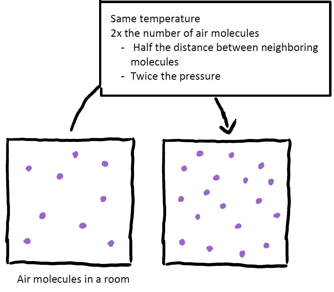
The air surrounding us consists primarily of tiny (\(\approx 1.5 \times 10^{-10} \:\mathrm{meters}\) in diameter) nitrogen molecules and oxygen molecules, which we will refer to collectively as “air molecules”, floating around in empty space and bumping into each other. Here a “bump” is when two molecules get close enough that the electrons of one molecule can “feel” the electrons of the other via their electric fields, thus repelling one another and sending the two molecules in opposite directions. These bumps are responsible for keeping the molecules afloat; the force behind these jolts is much stronger than the net gravitational pull that these molecules experience from the Earth, and so these interactions will repeatedly send molecules moving upwards, away from the ground (and those molecules that do hit the ground can bounce back up off of the ground’s molecules).
The effect of this constant jostling around is that, in the absence of any source of disturbance, air molecules will be roughly evenly spaced apart from one another. That is, if you were to go to your kitchen and measure the average distance between each air molecule and its nearest neighbor, and then repeat the process in your bed room, you would end up measuring nearly identical averages for the two rooms (if you live near sea level, then you would see that an air molecule can travel, on average, \(690 \times 10^{-10} \:\mathrm{meters}\) – about \(460\) times the size of its own diameter – before colliding with another air molecule). Put more concisely: the two rooms have the same uniform density of air molecules. We will see that the creation of a sound wave involves disturbing this even spacing.
“Air pressure” is likely a familiar phrase to us, although we might not have a precise understanding of what it is. The pressure of a gas (or a fluid) is a statistical measurement of the average force with which a gas presses against a surface; this is measured per unit of area of the surface. We can also understand this to be a measure of the average rate and strength with which the air molecules collide against a surface. Air pressure is thus, in part, a reflection of the average spacing between air molecules: the more tightly packed molecules are in a region of space, the more frequently they will collide with a given surface. This leads us to infer that pressure is inversely proportional to the average spacing between air molecules.
To see this, suppose that you have hermetically sealed off your bed room so that it is air tight. Now start pumping more air into your room (while holding its temperature fixed, which ensures that, on average, the particles are moving at the same speed as before) such that there are now twice as many air molecules in the room as when you started. With twice the number of particles in the same space, we can deduce that the average spacing between them will be half of what it was. Furthermore, a surface will experience twice the number of collisions, each of the same average strength as before, in a given amount of time. Thus we can conclude that the pressure in the room has doubled.
Given this relationship between the relative spacing of air molecules and the pressure that they exert, it should be clear that if a room has a uniform density of air molecules, we will find that there is a uniform air pressure throughout.
This discussion is meant to give us an understanding of the state of air in the absence of sound waves. That is, we have been building up some intuition for the medium through which sound travels. Next, we will learn that, when we sing or clap our hands, we are pushing on the air molecules around us and creating waves of high (and low) pressure, which zip through the air and cause our eardrums to vibrate.
Takeaway:
Air is a collection of gaseous molecules – primarily nitrogen and oxygen – that float through otherwise empty space and collide with one another repeatedly. These jostling molecules are roughly evenly distributed through space as long as no external source (e.g. an audio speaker) is disturbing them. This implies that the pressure, which measures the average rate and strength with which the molecules collide against a surface (per unit area), will be found to be constant throughout a room. The pressure and density of air are proportional: when we compress air (i.e. reduce the spacing between neighboring air particles), we increase both the pressure and density in that region.
We will see that sound waves perturb this uniformity: propagating regions of high and low air pressure are what our ears sense as auditory phenomena.
Sound Waves
We experience sound when regions of high air pressure and low air pressure crash up against our ear’s eardrum, causing it to flex inward (due to high pressure) and outward (due to low pressure). The vibration of one’s eardrum inward and outward is what drives the auditory sensation that enters into our consciousness as sound. These vibrations, as you likely know, are driven by sound waves.
Whenever we encounter any wavelike phenomenon in physics, be it water waves, seismic waves, electromagnetic waves or others, we should ask ourselves what thing is actually “waving” (oscillating). When it comes to sound waves, the quantity that is “waving” is the density of air, which, as we established above, is tantamount to saying that sound waves are traveling oscillations in air pressure. Let’s consider how these compression waves – propagating regions of high pressure (compressed) air and regions of low pressure (rarefied) air – get created.
A Clap
Clapping your hands together presses the air between your hands outwards. The air molecules evacuating from this space crash up against the neighboring molecules around your hand, creating an envelope of compressed (high density) air. As we discussed in the section above, this region of compression will have a higher pressure than the rest of the air in the room, whereas the evacuated space between your hands has a relatively low pressure (low density of air molecules). We say that this low density region is rarefied. These are the beginnings of a sound wave.
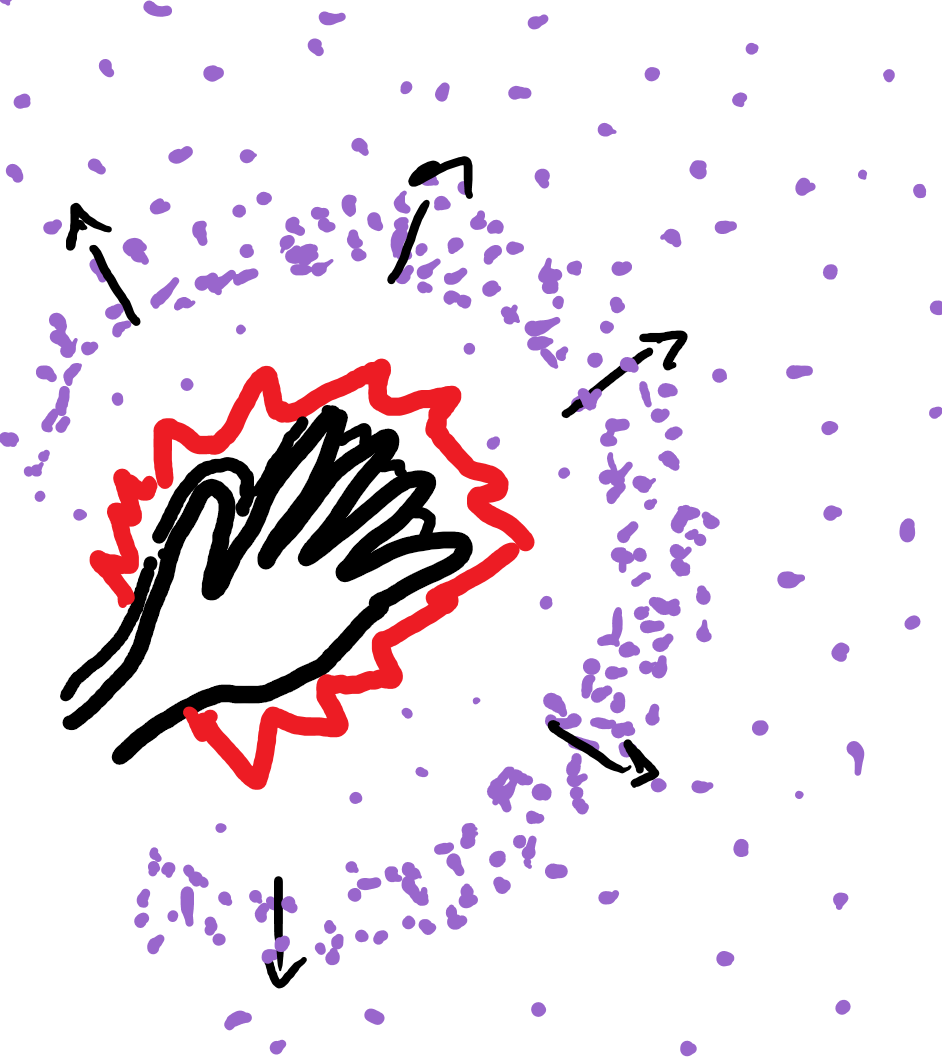
The compressed pocket of air surrounding your hands doesn’t remain compressed for long: the air molecules that were collided against get sent speeding outwards away from your hands, leaving a gap of rarefied air in their wake. These molecules surge outwards until they compress against their nearest neighbors. The region of high pressure (compressed air molecules) has effectively propagated outward, away from your hands. This domino effect continues, and an envelope of high-pressure air shoots outward throughout the room.
The room’s standing density of air molecules and temperature determine how quickly the air molecules will collide with each other, and thus determines how quickly this cascade of collisions will propagate through the room. At sea level and at room temperature (\(22 \:{}^\circ \mathrm{C}\) or \(72 \:{}^\circ \mathrm{F}\)), this envelope of compressed air will shoot outward at a speed of \(343 \:\frac{\mathrm{meters}}{\mathrm{second}}\), which is \(767 \:\frac{\mathrm{miles}}{\mathrm{hour}}\); this is the speed of sound.
When the propagating disturbance in the air reaches your ear, the high pressure air pushes your eardrum inward and the subsequent wake of low pressure air sucks it back outward. The disturbance in the air from your clap reverberates, causing multiple waves of high and low regions of pressure. Your eardrum vibrates back and forth because of this and a loud CLAP sounds in your consciousness. As the air around your ear settles down back to a state of uniform pressure (that is, the air pressure just outside your ear matches the pressure within your ear), your eardrum settles down and then you stop experiencing the sound of the clap.
The following plot depicts the measured fluctuations in air pressure, relative to the standing pressure in the room, of a single clap over time at one’s eardrum.
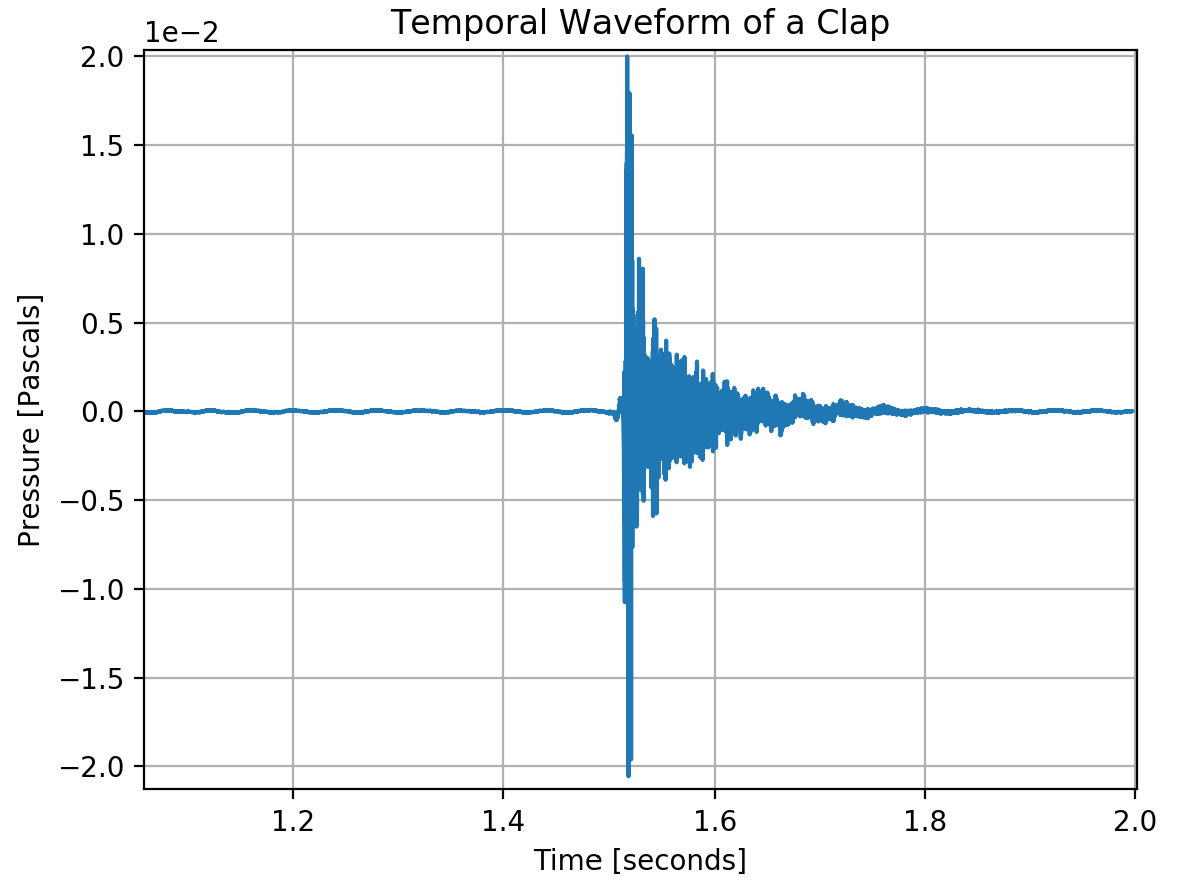
This plot is known as a temporal wave form, which we will discuss further later. Note that this was actually recorded by a microphone, which detects fluctuations in pressure similarly to our ears. The initial plateau of zero pressure indicates silence; there are no perceptible fluctuations in the air pressure. After waiting roughly \(1.5\) seconds someone clapped their hands and the resulting sound wave reached the eardrum, causing the large fluctuations seen in the plot. The large spike in pressure corresponds to the first wavefront of compressed air molecules crashing up against the eardrum. This is immediately followed by a low-pressure rarefaction, which is measured as negative pressure relative to the typical pressure in the room. Reverberations of high and low oscillations in air pressure continue to vibrate the ear drum, but these quickly become imperceptible as the magnitude of the fluctuations die down. After about \(0.2\) seconds, the air density fluctuations from the clap have all but ceased.
Let’s take a moment to see what the sound wave of a clap actually looks like (among other sources of sound). Please watch this brief video that was created by NPR. It may be worthwhile to re-read the preceding paragraphs after we watch this, so that we can reflect on the description of a clap’s compression wave along with the visuals that we see here:
Takeaway:
A sound wave is a type of compression wave. It is an oscillation in air density, and thus air pressure, that is spurred by collisions between molecules, which are driven by some mechanical impetus (e.g. clapping hands or a vibrating speaker). These collisions create regions of compressed (high density / pressure) air and leave gaps of rarefied (low density / pressure) air. Cascades of subsequent collisions are responsible for propagating these oscillations through the air; the speed with which the sound wave travels is determined primarily by the temperature and density of the air. At room temperature and at sea level, sound waves will propagate at a speed of \(343 \:\frac{\mathrm{meters}}{\mathrm{second}}\) \(\big(767 \:\frac{\mathrm{miles}}{\mathrm{hour}}\big)\).
The oscillating air pressure associated with a sound wave drives oscillations of one’s eardrums. This spurs our auditory system to perceive sound.
Quantifying Sound: Pure Tones
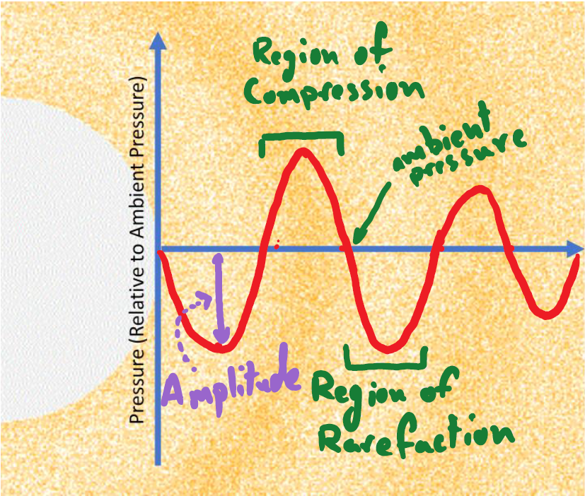
The following animation depicts a periodic sound wave emanating outward through the air from a central point. We can imagine that there is a speaker in the middle of the figure, which is responsible for driving these compression waves. Remember, the quantity that is oscillating here is air pressure (or, air density). Unlike water waves, the air molecules aren’t wobbling up and down, perpendicular to the wave’s plane of motion. Instead, these are “longitudinal” oscillations: the air compresses and rarefies along its direction of motion, like a Slinky. Let’s identify some essential quantities that we can use to characterize the simple sound wave being created by this speaker; we will measure the sound wave’s amplitude, frequency, and wavelength.
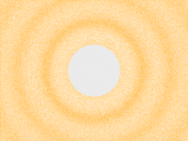
The regions of compression and rarefaction of this particular wave are oscillating sinusoidally – like a sine function – in both time and space. We will see that this is a very specific type of wave, which corresponds to the sound of a pure tone. The simplicity and regularity of this wave form will permit us to define the quantities of amplitude and frequency. Although a typical sound that we encounter in the real world (like the clap depicted above) is not a pure tone and thus cannot be characterized by a single sinusoid, pure tones will serve to be indispensable constructs for analyzing “realistic” sounds later on.
Spatial Waveforms
The following plot is the spatial waveform of the sound wave: it depicts and quantifies the spatial variation of air pressure due to a sound wave in a fixed moment of time (see that it is plotted against a single frame from the preceding animation).
The x-axis of this plot conveys a spatial dimension and carries units of length (e.g. meters).
We can represent a simplified, one-dimensional version of this spatial wave form as
The wave’s amplitude, \(A\), is the absolute value of the “gauge” pressure associated with most highly-compressed, or most rarefied, region of the sound wave: it is measured relative to the standing air pressure in the absence of any disturbances. Note that, in actuality, the amplitude of this wave decays as it moves away from the speaker; we are glossing over this detail with our mathematics here. This is always recorded as positive quantity, regardless of if you are measuring the pressure at a peak (compression) or trough (rarefaction), and it carries the units of pressure (force per unit area, or Pascals). When a sound wave strikes our ear, its amplitude impacts the magnitude with which one’s eardrum gets pushed on. A high-amplitude wave causes heavily compressed (high pressure) air to push hard on our eardrum and starkly rarefied (low pressure) air to pull strongly on it. This manifests in our perception of sound as loudness. That is, a sound wave with a large amplitude will sound louder to us than a sound wave with a small amplitude.
Aside:
While we describe the amplitude of a pressure wave in units of Pascals, in every-day life, we more frequently see decibels, denoted \(\mathrm{dB}\), used to describe the loudness of a sound.
Decibels are a (base \(10\)) logarithmically scaled unit used to measure how loud we perceive sounds. In particular, incrementing the loudness of a noise by \(1\) decibel actually corresponds to the amplitude of the pressure wave increasing by a factor of about \(1.122\). So, if a song were playing at \(50\:\mathrm{dB}\), and someone cranked up the volume to \(100\:\mathrm{dB}\), the actual amplitude of whatever pressure wave our ears detected would not have simply doubled. In fact, the amplitude would have increased by a factor of approximately \(316\).
Decibels are an extremely convenient measure of volume because our hearing actually operates on a logarithmic scale. This means that if we heard a song turned up from \(50\:\mathrm{dB}\) to \(100\:\mathrm{dB}\), we would perceive this change as the volume doubling and not as the volume increasing by a factor of \(316\). Consequently, it is often much more convenient to describe the loudness sounds with decibels than Pascals. That being said, when we talk about pressure mathematically, we ought to use the true units of pressure, Pascals.
The wavelength of this sound wave, denoted by \(\lambda\), is the distance between two consecutive peaks (or troughs) in the sinusoid; it carries units of length (e.g. meters). We will discuss wavelength further in a moment. However, for our purposes, we will be working with temporal wave forms and not spatial ones.
Temporal Waveforms
A temporal wave form is a plot of the variation in air pressure over time, at a single point in space. We already looked at the temporal wave form for a clap in the previous section. The x-axis of this plot is the temporal dimension and thus carries units of time (e.g. seconds). The temporal wave form for this wave is described by
Notice that, because we are describing the pressure fluctuations over time at a fixed location (e.g. at a microphone), time, \(t\), is the only variable in this equation. For simplicity, we have also assumed that \(p(0)=0\), which is why we used sine instead of cosine and did not include a phase-shift term. Let’s break down this equation.
The wave’s frequency, \(f\), is a measure of how quickly the wave form repeats itself in time. Frequency is measured as the number of oscillations (repetitions), which is a unitless quantity, per unit time. We will be dealing with number of oscillations per second, which is known as Hertz and is abbreviated as \(\mathrm{Hz}\). To determine the frequency of the wave animated above, place your cursor (or finger) over a fixed position on the animation. Set a timer on your phone for some brief interval of time – let’s say 15 seconds. We will count the number of peaks that pass through our cursor during that interval. About five peaks should pass over our cursor during this interval, which means that this compression wave is oscillating at a frequency of \(\frac{5\:\mathrm{oscillations}}{15\:\mathrm{seconds}}\), or \(0.33 \:\mathrm{Hz}\). We multiply \(f\) by \(2\pi\) because the sine function must have as its input a number in radians, and it completes one oscillation for every \(2\pi\) radians: \(\big(\frac{\mathrm{radians}}{\mathrm{oscillations}}\big)\big(\frac{\mathrm{oscillations}}{\mathrm{seconds}}\big)\,\mathrm{seconds} \rightarrow \mathrm{radians}\).
The soundwave’s frequency determines the rate at which one’s eardrum vibrates, which we perceive as pitch. Sound waves whose compression cycles oscillate at a high frequency rattle our eardrums rapidly, which causes us to hear a high-pitch noise, whereas low-frequency sound waves sound like a low-pitch noise. However, humans don’t perceive all vibrations to our eardrums; we perceive sound wave that oscillate between twenty oscillations per second (\(20 \:\mathrm{Hz}\)), and twenty thousand oscillations per second (\(20,000 \:\mathrm{Hz}\), or \(20 \:\mathrm{KHz}\)). Thus the sound wave depicted above would actually be imperceptible to us since it oscillates at roughly \(0.33 \:\mathrm{Hz}\); it does not vibrate our eardrums quickly enough to be perceived.
Reading Comprehension: Temporal Waveform:
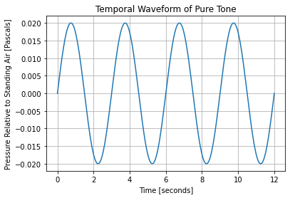
Using the matplotlib library, plot the temporal waveform for the pure tone that is animated above, for a span of \(12\) seconds. Assume that we measure an amplitude of \(0.02\) Pascals and use the frequency that we measured above. The y-axis should have units of Pascals and the x-axis should carry units of seconds. Use ax.set_ylabel() and ax.set_xlabel(), respectively, to label the axes of your
plot.
What should the time-length be between the consecutive peaks in your plot?
The Relationship Between Frequency and Wavelength
As described above, the wavelength, \(\lambda\), of a pure tone measures how far apart two consecutive pressure peaks are in space. The frequency, \(f\), measures the rate at which peaks pass through a given point in space. Thus the product of these two quantities yield the speed with which the wave is propagating through space – the distance traveled by a region of compression in a given amount of time:
But, as we established above, the speed of sound is fixed by the properties of the medium through which it travels (air). At room temperature and the atmospheric pressure associated with sea-level, the speed of sound is the fixed value
Thus the frequency and wavelength of a sound wave are mutually determined: if you know the wave’s frequency, then its wavelength is fixed by the relationship
and vice versa. Note that dividing \(\frac{\mathrm{meters}}{\mathrm{second}}\) by \(\frac{1}{\mathrm{second}}\), or \(\mathrm{Hz}\), yields \(\mathrm{meters}\).
Reading Comprehension: Wavelength and Frequency:
Based on our discussion of the interdependency of wavelength and frequency, and assuming that we are at sea-level and at room temperature:
What is the wavelength of the animated sinusoidal sound wave above (in meters)?
Given that we hear pure tones in the range of frequencies \([20\:\mathrm{Hz}, 20,000\:\mathrm{Hz}]\), what are the wavelengths associated with these bounds (in meters)?
Takeaway:
A pure tone is a sound wave whose regions of compression and rarefaction oscillate sinusoidally in space and time. This simple and orderly wave form has a well defined amplitude, which is the magnitude of the discrepancy between the maximum (or minimum) pressure of the compression wave and pressure of the surrounding air, measured in Pascals. A sound wave’s amplitude determines the loudness that we perceive. A pure tone also has a well-defined frequency, which is the rate at which points of maximum pressure pass through a point in space, measured in Hertz (\(\mathrm{Hz}\)). The frequency of the sound wave determines the sound’s pitch that we perceive.
The speed of any sound wave is determined by the pressure and temperature of the air through which it travels. Thus the wavelength of a pure tone – the distance between two consecutive pressure peaks in space – defines the tone’s frequency, and vice versa, via the relationship: \(\lambda = \frac{v_\text{sound}}{f}\)
Realistic Sounds and the Principle of Superposition
It is critical to note that the quantities introduced in this section – amplitude and frequency – and the sinusoidal temporal waveform written above do not directly describe the sounds that we typically hear. As we saw earlier, a single clap does not produce a wave form that repeats periodically for all time, nor does its waveform possess peaks of a uniform amplitude that recur at a single frequency. Furthermore, the sounds that we hear have more perceptual nuances to them than mere loudness and pitch – the timbre and sonic texture of a sound wave helps to describe the difference in quality of, say, a C5 note played on a piano versus one played on a guitar.
That being said pure tones (sinusoidal waveforms) are not merely things of pedagogy; it turns out that even the most disorderly sounds can be decomposed into a combination of (infinitely many) pure tones. This insight is the crux of nearly all audio analysis techniques and is a topic that we will study in detail in the coming sections of this module. To understand what is meant by “decomposed”, let’s briefly discuss what it means to compose, or combine, sounds together.
Suppose that we have two loud speakers, \(A\) and \(B\), playing two separate songs. Let the pressure fluctuations of the sound wave coming from speaker \(A\) be described by the function \(p_A(x, t)\) (we are restricting ourselves to one spatial dimension here), and those of speaker \(B\) be given by \(p_B(x, t)\). Then the function describing the combined sound wave resulting from the two speakers is simply
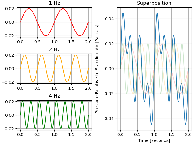
The fact that we simply add the speakers’ respective sound waves together to describe the resulting total sound wave is quite remarkable. Based only on our discussion thus far, there was nothing guaranteeing this tidy behavior; it very may well have been the case that the individual waves combine through some complicated multiplicative process. That sound waves combine together via simple additions is known as the principle of superposition; this property is the result of the mechanical interactions between air molecules en masse. Superposition is a broad principle from physics that describes all so-called linear systems. The following plot depicts the superposition of three temporal wave forms, which oscillate at \(1\:\mathrm{Hz}\), \(2\:\mathrm{Hz}\), and \(4\:\mathrm{Hz}\) respectively.
Aside (Advanced):
A note for those readers with a more extensive background in mathematics: the differential equation that describes the spatio-temporal dynamics of air density – the “wave equation” for sound – is linear. This means that the sum of any solutions to this differential equation is itself a solution (under the composition of their initial conditions). This is why sound waves obey the principle of superposition. That is, it is why we can separately solve the differential equation given the individual boundary conditions of the respective speakers and simply add their solutions to arrive at the culminating sound wave. Don’t worry if this paragraph sounded like gibberish.
Takeaway:
Sound waves obey the principle of superposition, which means that the sound waves emanating from different sources interact with each other by simply adding their fluctuations in air pressure together. That is, if the \(0.01\) Pascal pressure peak of one wave overlaps (in space and time) with the \(0.03\) Pascal pressure peak of another sound wave, the resulting pressure at the point and time will be \(0.04\) Pascals. With the principle of superposition in mind, we will analyze complex sounds by representing them as the summation of many simple, pure tones.
Reading Comprehension Exercise Solutions
Temporal Waveform: Solution
Using the matplotlib library, plot the temporal waveform for the pure tone that is animated above, for 12 seconds. Assume that we measure an amplitude of \(0.02\) Pascals and use the frequency that we measured above.
First we need to create an array of time values that we can use to “sample” our temporal wave form over the 12 second interval. Let’s evenly sample the domain \([0, 12)\) with \(1,000\) points so that our plot looks nice and smooth
import numpy as np

# evenly sample 1000 times from 0 seconds to 12 seconds
times = np.linspace(0, 12, 1000)  # seconds; shape-(1000,)
Now we’ll “measure” the pressure of the sinusoidal waveform at each of these times. We’ll leverage NumPy’s vectorized operations to do this succinctly – no for-loops for us!
freq = 1 / 3  # Hertz
amp = 0.02  # Pascals
pressures = amp * np.sin(2 * np.pi * freq * times)  # Pascals; shape-(1000,)
What should the time-length be between the consecutive peaks in your plot?
Frequency, \(f\), measures the number of repetitions per second, and thus its inverse, \(T = \frac{1}{f}\), measures the time between repetitions. This quantity is known as the wave’s period. Thus we should see that there is a \(T = 3\:\mathrm{seconds}\) gap between peaks in our wave form.
Let’s plot our temporal waveform:
[1]:
import matplotlib.pyplot as plt
%matplotlib inline

import numpy as np

# evenly sample 1000 times from 0 seconds to 12 seconds
times = np.linspace(0, 12, 1000)  # seconds; shape-(1000,)

# measuring pressure at the specified times
freq = 1 / 3  # Hertz
amp = 0.02  # Pascals
pressures = amp * np.sin(2 * np.pi * freq * times)  # Pascals; shape-(1000,)

fig, ax = plt.subplots()

ax.plot(times, pressures)
ax.set_xlabel("Time [seconds]")
ax.set_ylabel("Pressure Relative to Standing Air [Pascals]")
ax.set_title("Temporal Waveform of Pure Tone")
ax.grid(True)
Wavelength and Frequency: Solution
What is the wavelength of the animated sinusoidal sound wave above (in meters)?
We measured the animated wave’s frequency to be approximately \(0.33\:\mathrm{Hz}\). Given that this is a sound wave, we know its speed. Thus its wavelength is \(\frac{343 \:\frac{\mathrm{meters}}{\mathrm{second}}}{0.33\:\mathrm{Hz}} = 1,040 \:\mathrm{meters}\). This means that the length scale depicted in the animation is quite large – the full image is roughly \(6,000 \:\mathrm{meters}\) across.
Given that we hear pure tones in the range of frequencies is \([20\:\mathrm{Hz}, 20,000\:\mathrm{Hz}]\), what are the wavelengths associated with these bounds (in meters)?
The wavelength is inversely proportional to the frequency, so the ordering of the bounds on wavelength have their order reversed: the high-frequency bound corresponds to the short-wavelength bound.